Accelerating Drug Discovery: How Automated Forcefield Parameterization Predicts Glass Transition Temperature (Tg)
This article explores the transformative role of automated forcefield parameterization in predicting the glass transition temperature (Tg) of amorphous solid dispersions and polymeric excipients.
Accelerating Drug Discovery: How Automated Forcefield Parameterization Predicts Glass Transition Temperature (Tg)
Abstract
This article explores the transformative role of automated forcefield parameterization in predicting the glass transition temperature (Tg) of amorphous solid dispersions and polymeric excipients. Aimed at researchers and pharmaceutical developers, we first establish the foundational importance of Tg for drug stability and manufacturability, then detail cutting-edge methodologies from machine learning-assisted fitting to high-throughput workflows. The guide provides actionable solutions for common parameterization pitfalls and compares leading validation frameworks. Ultimately, we demonstrate how this computational acceleration de-risks formulation development and paves the way for more robust, stable drug products.
Why Tg Matters: The Critical Link Between Glass Transition, Drug Stability, and Molecular Dynamics
The glass transition temperature (Tg) is a critical material property in pharmaceutical science, dictating the physical stability, dissolution behavior, and shelf-life of amorphous solid dispersions, freeze-dried products, and polymeric excipients. Within the thesis on Automated forcefield parameterization for Tg prediction research, accurately defining and measuring Tg is the essential experimental benchmark. This protocol details the core principles, measurement techniques, and data interpretation required to robustly characterize Tg, providing the necessary ground truth for validating computational predictions from automated forcefield pipelines.
Core Principles and Data
The glass transition is a kinetic phenomenon, observed as a reversible change in the thermal and mechanical properties of an amorphous material upon heating or cooling. The measured Tg value depends on the experimental timescale (scan rate) and the material's thermal history.
Table 1: Key Quantitative Parameters for Pharmaceutical Tg Analysis
| Parameter | Typical Range (Pharmaceuticals) | Significance |
|---|---|---|
| Measured Tg | 50°C to 180°C (for common polymers & APIs) | Primary indicator of physical stability. Higher Tg generally implies greater kinetic stability. |
| ΔCp at Tg | 0.1 to 0.5 J g⁻¹ K⁻¹ | Heat capacity jump. Related to the gain in conformational degrees of freedom. |
| Fragility Index (m) | ~50 (Strong) to ~150 (Fragile) | Describes how sharply viscosity changes with T near Tg. Critical for predicting stability under varying storage conditions. |
| Kauzmann Temperature (T₀) | Typically Tg - 20°C to Tg - 50°C | Theoretical temperature of zero configurational entropy. A key target for thermodynamic models. |
| Critical Cooling Rate (q_c) | 10² to 10⁵ K/s | Minimum cooling rate to avoid crystallization. Informs process design (e.g., melt quenching, spray drying). |
Experimental Protocols
Protocol 3.1: Differential Scanning Calorimetry (DSC) for Tg Determination
Principle: Measures the difference in heat flow between a sample and an inert reference as a function of temperature, detecting the heat capacity change at Tg.
Materials:
- Hermetically sealed aluminum DSC pans and lids
- Analytical balance (µg precision)
- Nitrogen purge gas (50 mL/min)
Procedure:
- Sample Preparation: Pre-dry the amorphous solid. Precisely weigh 3-10 mg of sample into a tared DSC pan. Crimp the lid to ensure a hermetic seal.
- Instrument Calibration: Calibrate the DSC for temperature and enthalpy using indium and zinc standards.
- Method Programming:
- Equilibrate at 20°C below the expected Tg.
- Isothermal hold for 5 min to erase thermal history.
- Heat at a standard rate of 10 K/min to at least 30°C above Tg.
- Cool at 20 K/min to starting temperature.
- Repeat the heating scan (2nd heat) at 10 K/min for analysis.
- Data Analysis: Analyze the second heating curve. Tg is reported as the midpoint of the step change in heat flow (extrapolated onset and endpoint should also be noted).
Protocol 3.2: Dynamic Mechanical Analysis (DMA) for Tg Determination
Principle: Applies an oscillatory stress to the sample and measures the resultant strain, determining the viscoelastic moduli (Storage (E') and Loss (E'') moduli). Tg is identified from the peak in tan δ (E''/E') or the onset of the drop in E'.
Materials:
- DMA equipped with film tension or compression clamps
- Amorphous film or compacted powder sample
Procedure:
- Sample Preparation: Prepare a free-standing film or a uniformly compressed powder disk of known geometry (length, width, thickness).
- Mounting: Clamp the sample securely, ensuring good contact without over-torquing.
- Method Programming:
- Set a static force/strain within the linear viscoelastic region.
- Apply a sinusoidal oscillation at a fixed frequency (e.g., 1 Hz).
- Ramp temperature at 3 K/min over a suitable range.
- Data Analysis: Identify Tg as the temperature at the peak of the tan δ curve. Report the frequency used.
The Scientist's Toolkit: Research Reagent Solutions
Table 2: Essential Materials for Tg Research
| Item | Function/Application |
|---|---|
| Amorphous Pharmaceutical Polymer (e.g., PVP-VA, HPMC-AS) | Model polymer for forming solid dispersions. High Tg impacts API stabilization. |
| Hermetic Sealed DSC Pans (Tzero recommended) | Ensures no mass loss (solvent, decomposition) during heating, crucial for accurate ΔCp measurement. |
| Standard Reference Materials (Indium, Zinc, Sapphire) | Calibration of DSC temperature, enthalpy, and heat capacity, respectively. |
| Quartz or Aluminum DMA Clamps | Provide inert, rigid mounting surfaces for film/disk samples in DMA. |
| Controlled Humidity Chamber | For preconditioning samples at specific %RH to study plasticization by water (critical for Tg prediction). |
| High-Purity Nitrogen Gas | Inert purge gas for DSC/TGA to prevent oxidative degradation during heating. |
| Fast-Scan DSC Chip Sensor | Enables cooling/heating rates >100 K/min to study intrinsic material behavior near the critical cooling rate. |
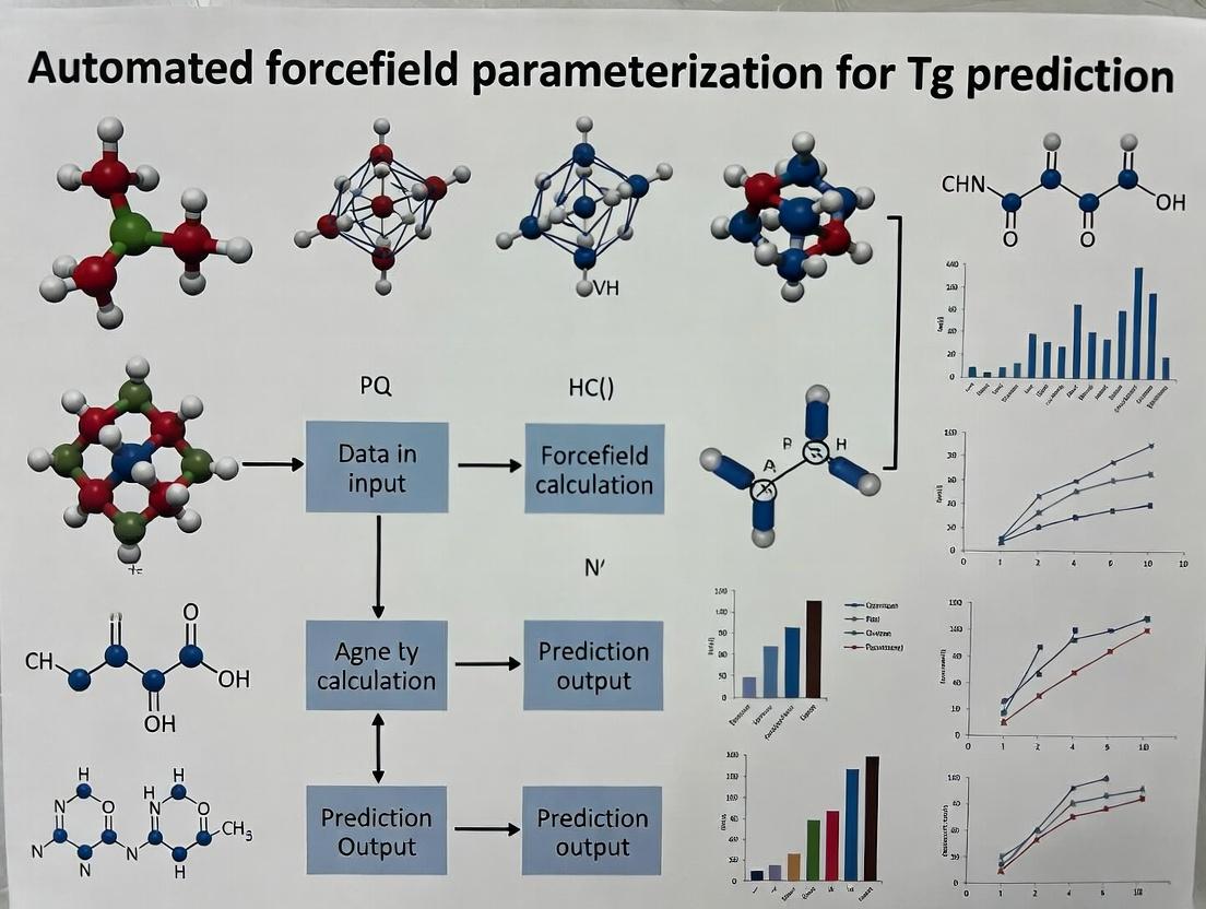
Visualization of Concepts and Workflows
Diagram 1: Tg Research in Forcefield Parameterization
Diagram 2: Standard DSC Protocol Steps
Diagram 3: Factors Influencing Measured Tg
This document outlines key experimental protocols and data within the broader research thesis on Automated forcefield parameterization for Tg prediction. The accurate prediction of the glass transition temperature (Tg) is critical for the rational design of amorphous solid dispersions (ASDs), biologics formulations, and other systems where physical stability, crystallization propensity, and shelf life are governed by molecular mobility below and above the Tg.
Table 1: Tg Values and Stability Correlates for Common Pharmaceutical Polymers and Formulations
| Material/System | Measured Tg (°C) | Critical ∆T (T - Tg) for Onset of Instability | Estimated Relaxation Time at 25°C (τ, s) | Observed Crystallization Onset (Accelerated Conditions) |
|---|---|---|---|---|
| Pure PVP VA64 | 106 | +50°C | >10^7 | N/A (stable) |
| Pure HPMCAS | 120 | +55°C | >10^8 | N/A (stable) |
| Itraconazole: HPMCAS (30:70) ASD | 95 | +40°C | ~10^5 | 4 weeks (40°C/75% RH) |
| Sucrose (Pure) | 70 | +20°C | ~10^2 | <1 day (40°C/dry) |
| Monoclonal Antibody (high conc.) | ~10 to 20 | +10°C | Varies with excipients | Aggregation onset >Tg |
Table 2: Key Input Parameters for Automated Forcefield Parameterization for Tg Prediction
| Parameter Class | Specific Variables | Target Experimental Data for Validation | Typical Range/Values |
|---|---|---|---|
| Bonded Terms | Bond stiffness (k), Equilibrium length | Vibrational spectroscopy (IR, Raman) | k: 200-600 kcal/mol/Ų |
| Non-bonded Terms | Partial atomic charges, LJ epsilon & sigma | Heat of vaporization, Density, Dielectric constant | ε: 0.05-0.3 kcal/mol, σ: 3.0-4.5 Å |
| Dihedral Terms | Rotational barriers, Multiplicity | Conformational energy profiles (QM) | Barrier: 0.5-3.0 kcal/mol |
| System Control | Cooling rate (computational) | Experimental DSC cooling rate (validated) | 1-100 K/ns (comp) vs. 0.5-20 K/min (exp) |
Experimental Protocols
Protocol 1: Determination of Tg via Differential Scanning Calorimetry (DSC)
Objective: To measure the experimental glass transition temperature of a candidate amorphous material for forcefield validation.
Materials:
- TA Instruments Q2000 DSC or equivalent.
- Tzero aluminum pans and lids.
- Microbalance (±0.001 mg).
- Sample (5-10 mg, lyophilized or melt-quenched).
- Liquid Nitrogen Cooling System.
Procedure:
- Sample Preparation: Pre-dry sample if hygroscopic. Pre-dry pans/lids at relevant temperature.
- Loading: Precisely weigh 5-10 mg of sample into a Tzero pan. Crimp the lid non-hermetically.
- Method Programming:
- Equilibrate at 20°C below expected Tg.
- Ramp 10.00°C/min to 30°C above expected degradation/melt temperature.
- Isothermal for 5 min to erase thermal history.
- Quench cool at 50°C/min to 20°C below expected Tg.
- Ramp 10.00°C/min for second heat (analysis cycle).
- Data Analysis: Use TA Universal Analysis software. Tg is identified as the midpoint of the heat capacity step change in the second heating cycle. Report onset, midpoint, and endpoint.
Protocol 2: Molecular Dynamics (MD) Simulation for Tg Prediction
Objective: To computationally predict Tg using candidate automated forcefields.
Materials:
- High-performance computing cluster.
- Simulation software (GROMACS, LAMMPS, Desmond).
- Initial molecular structure files (e.g., .pdb, .mol2).
- Forcefield parameter files (generated from automated pipeline).
- Analysis scripts (Python, VMD, MDAnalysis).
Procedure:
- System Construction: Build an amorphous cell of ~100 molecules using Packmol. Ensure density is slightly below experimental room-temperature density.
- Energy Minimization: Minimize using steepest descent algorithm until Fmax < 1000 kJ/mol/nm.
- Equilibration (NPT):
- Run at 500 K (well above expected Tg) for 5 ns using Nose-Hoover thermostat (τ=1 ps) and Parrinello-Rahman barostat (τ=5 ps, 1 atm).
- Ensure density fluctuates around stable mean.
- Cooling Run: Using the equilibrated configuration, run a simulated cooling scan.
- Decrease temperature in 10-20 K decrements from 500 K to 200 K.
- At each temperature, run a 2-5 ns NPT simulation (same settings as step 3).
- Save the final configuration of each step as the start for the next.
- Data Analysis: For each temperature step, calculate the average specific volume (or density) over the final 1 ns of simulation. Plot specific volume vs. Temperature. Fit lines to the high-T (rubbery) and low-T (glassy) regions. The intersection defines the predicted Tg.
Protocol 3: Stability Study for Crystallization Onset
Objective: To empirically determine the relationship between storage temperature (T), Tg, and crystallization onset time.
Materials:
- Stability chambers (controlled temperature ±0.5°C, humidity ±2% RH).
- X-ray Powder Diffractometer (XRPD).
- DSC (from Protocol 1).
- Sample vials with controlled humidity seals.
Procedure:
- Sample Conditioning: Prepare identical amorphous samples (e.g., spray-dried ASD). Characterize initial state (Tg via DSC, amorphousness via XRPD).
- Storage Matrix: Place samples in stability chambers at temperatures T such that ∆T = (T - Tg) = 10, 20, 30, 40, and 50°C. For hygroscopic samples, control RH at 0% (dry) or a relevant humidity (e.g., 75% RH).
- Sampling Schedule: Withdraw samples at logarithmic time intervals (e.g., 1 day, 3 days, 1 week, 2 weeks, 1 month, 3 months, 6 months).
- Analysis: For each time point:
- Perform XRPD to detect crystalline peaks. The onset time is when characteristic peaks exceed baseline noise by 3σ.
- Perform DSC to monitor any change in Tg and detect melting events of crystalline material.
- Modeling: Plot log(crystallization onset time) vs. 1/(∆T) or fit to the Williams-Landel-Ferry (WLF) equation.
Visualizations
Workflow for Automated Tg Prediction
Tg Governs Stability via Molecular Mobility
The Scientist's Toolkit: Research Reagent Solutions
Table 3: Essential Materials for Tg and Stability Research
| Item | Function/Relevance |
|---|---|
| Differential Scanning Calorimeter (DSC) | Gold-standard for experimental Tg measurement via heat capacity change. |
| Molecular Dynamics Software (GROMACS/LAMMPS) | Platform for running cooling simulations to predict Tg from forcefields. |
| High-Performance Computing Cluster | Necessary for the computationally intensive MD simulations of large, amorphous systems. |
| Quantum Mechanics Software (Gaussian, ORCA) | Used to generate target data (charges, torsion profiles) for forcefield parameterization. |
| Amorphous Solid Dispersion (ASD) Libraries | Pre-formulated ASDs of API with polymers (PVP, HPMCAS) for experimental benchmarking. |
| Controlled Humidity/Temperature Stability Chambers | For empirical stability studies linking ΔT to crystallization/aggregation onset. |
| X-ray Powder Diffractometer (XRPD) | Critical for confirming amorphous state and detecting crystallinity during stability tests. |
| Parameter Optimization Algorithm (e.g., ForceBalance) | Software that automates the iterative fitting of forcefield parameters to experimental data. |
This application note details the critical role of molecular mechanics force fields in bridging atomistic simulations to macroscopic material properties, specifically the glass transition temperature (Tg). It supports the broader thesis on Automated forcefield parameterization for Tg prediction research by establishing the foundational protocols and validation metrics required to develop and assess force fields for amorphous solid dispersions in pharmaceutical development.
The Forcefield Paradigm: Equations and Parameters
A forcefield is a collection of mathematical functions and parameters that approximate the potential energy (U) of a molecular system. The accuracy of property prediction is directly contingent on the fidelity of these terms.
Total Energy Equation:
U_total = Σ_bonds K_r(r - r0)^2 + Σ_angles K_θ(θ - θ0)^2 + Σ_dihedrals (K_φ/2)[1 + cos(nφ - δ)] + Σ_nonbonded {4ε[(σ/r)^12 - (σ/r)^6] + (q_i q_j)/(4πϵ_0 r)}
Table 1: Core Forcefield Components and Their Impact on Tg Prediction
| Component | Mathematical Form | Key Parameters | Role in Tg/Amorphous Properties |
|---|---|---|---|
| Bond Stretching | Harmonic: K_r(r - r0)^2 | K_r (force constant), r0 (eq. length) | Governs high-frequency vibrations; minor direct Tg impact. |
| Angle Bending | Harmonic: K_θ(θ - θ0)^2 | K_θ (force constant), θ0 (eq. angle) | Affects local chain stiffness; influences segmental mobility. |
| Torsional Rotation | Periodic: K_φ[1+cos(nφ-δ)] | K_φ (barrier height), n (periodicity), δ (phase) | CRITICAL. Dictates rotational energy barriers, directly controlling backbone flexibility and Tg. |
| van der Waals | Lennard-Jones: 4ε[(σ/r)^12-(σ/r)^6] | ε (well depth), σ (contact distance) | Governs intermolecular packing, cohesion energy density, and free volume. |
| Electrostatics | Coulomb: (qi qj)/(4πϵ_0 r) | qi, qj (partial atomic charges) | Determines inter/intra-molecular polarity, hydrogen bonding, and phase miscibility. |
Protocol: Molecular Dynamics Workflow for Tg Prediction
This protocol outlines the standard procedure for predicting Tg using molecular dynamics (MD) simulation, serving as the benchmark for evaluating automated parameterization methods.
A. System Preparation & Forcefield Assignment
- Build Amorphous Cell: Using software like Packmol or Materials Studio Amorphous Cell, construct a simulation box containing 20-50 polymer chains (or API/polymer mixtures) with periodic boundary conditions. Target density ~0.8-0.9 g/cm³.
- Assign Forcefield: Apply the chosen forcefield (e.g., GAFF2, OPLS-AA, CGenFF) using tools like
antechamber(for GAFF) or the software’s parametric assignment. Critical Step: Document all assigned parameters, especially torsional and non-bonded terms. - Energy Minimization: Perform steepest descent/conjugate gradient minimization (5000 steps) to relieve severe atomic clashes.
B. Equilibration Protocol (NPT Ensemble)
- Initial Thermalization: Run NVT simulation for 100 ps at 500 K (well above Tg) using a Langevin thermostat (damping constant 1 ps⁻¹).
- Density Equilibration: Switch to NPT ensemble (Nosé-Hoover barostat, target pressure 1 atm) at 500 K for 2-5 ns. Monitor density convergence.
- Stepwise Cooling: In the NPT ensemble, cool the system in 20-50 K decrements from 500 K to 200 K. At each temperature, run for 2-5 ns, ensuring properties (energy, density) stabilize.
C. Production Run & Tg Calculation
- Density vs. Temperature Sampling: After equilibration at each temperature in the cooling cycle, run a 5-10 ns NPT production simulation. Log the average density and specific volume.
- Data Analysis: Plot specific volume (or density) versus temperature. Fit linear regressions to the high-T (rubbery) and low-T (glassy) data.
- Tg Determination: Identify the intersection point of the two linear fits. This temperature is the simulated Tg. Report the slope ratio (expansion coefficient change).
Table 2: Typical Simulation Parameters & Expected Outcomes
| Parameter | Typical Value/Choice | Justification |
|---|---|---|
| Time Step | 1 fs | Stability with explicit atom detail and H-bonding. |
| Cut-off Radius | 10-12 Å for vdW & Coulomb (short-range) | Computational efficiency. |
| Long-Range Electrostatics | Particle Mesh Ewald (PME) | Accurate treatment of Coulomb forces. |
| Thermostat | Nosé-Hoover/Langevin | Proper canonical ensemble sampling. |
| Barostat | Parrinello-Rahman/Nosé-Hoover | Proper isotropic pressure control. |
| Expected Tg Error (vs. Exp.) | ±15-30 K (Classical FF) | Baseline for automated parameterization to improve upon. |
Visualization: Tg Prediction Workflow & Forcefield Dependence
Diagram 1: Forcefield-Driven Tg Prediction Workflow (93 chars)
Diagram 2: Key Forcefield Parameters Controlling Tg (91 chars)
The Scientist's Toolkit: Research Reagent Solutions
Table 3: Essential Materials & Software for Forcefield-Based Tg Research
| Item Name | Type/Category | Function in Research |
|---|---|---|
| General AMBER Force Field 2 (GAFF2) | Parameter Set | A widely used forcefield for organic molecules; baseline for automated small molecule parameterization. |
| Optimized Potentials for Liquid Simulations (OPLS-AA) | Parameter Set | A high-quality forcefield for biomolecules and organic liquids; standard for pharmaceutically relevant systems. |
| CHARMM General Force Field (CGenFF) | Parameter Set | A consistent forcefield with extensive biomolecular parameters; includes polymerizable residues. |
| Polymer Consistent Force Field (PCFF) | Parameter Set | A class II forcefield specifically optimized for polymers and inorganic materials. |
| GROMACS | MD Simulation Software | High-performance, open-source MD engine ideal for large-scale cooling and equilibration protocols. |
| LAMMPS | MD Simulation Software | Extremely flexible MD code with extensive coarse-graining and custom potential options. |
| Paramfit / ForceBalance | Parameterization Tool | Software for systematically deriving/optimizing forcefield parameters against quantum mechanical (QM) data. |
| Packmol | System Builder | Tool for building initial configurations of complex amorphous molecular mixtures. |
| MATLAB/Python (w/ NumPy, SciPy) | Data Analysis | Critical for scripting analysis of volumetric data, performing linear fits, and calculating Tg. |
1. Introduction & Thesis Context Within the broader thesis on "Automated forcefield parameterization for Tg prediction research," a critical challenge is the accurate and efficient derivation of molecular mechanics parameters for complex Active Pharmaceutical Ingredients (APIs) and amorphous polymeric excipients. The glass transition temperature (Tg) is a crucial property influencing drug stability, dissolution, and shelf-life. Accurate prediction via molecular dynamics (MD) simulations depends entirely on the quality of the forcefield parameters. This document details application notes and protocols comparing manual and automated parameterization approaches, providing a framework for researchers in computational pharmaceutics and drug development.
2. Comparative Analysis: Manual vs. Automated Parameterization
Table 1: Comparison of Manual vs. Automated Parameterization Approaches
| Aspect | Manual Parameterization | Automated Parameterization (e.g., using FFToolkit, MATCH, GAAMP, CGenFF) |
|---|---|---|
| Core Methodology | Literature survey, QM target data calculation (geometry, ESP, torsional scans), iterative fitting to match QM/experimental data. | Rule-based assignment from analogy, systematic optimization algorithms (e.g., Monte Carlo, genetic algorithms) to minimize error vs. QM data. |
| Time Investment | Weeks to months per novel molecule. | Hours to days per molecule, after initial setup. |
| Required Expertise | Very high (QM, forcefield theory, scripting). | Moderate (software proficiency, basic forcefield knowledge). |
| Transferability | High, if principles are rigorously applied. | Variable; depends on parent forcefield and training set coverage. |
| Consistency | Prone to human error and subjective decisions. | High, as the same protocol is applied uniformly. |
| Best For | Novel molecular scaffolds, critical torsion parameters, final validation. | High-throughput screening, homolog series, initial parameter generation. |
| Typical RMSE vs. QM Torsional Scans | 0.2 - 0.5 kcal/mol (with careful fitting). | 0.5 - 1.5 kcal/mol (can be lower with advanced optimization). |
| Integration with Tg Workflow | Bottleneck; limits system size and throughput. | Enables high-throughput generation of parameters for polymer/API blends for Tg prediction. |
3. Application Notes & Detailed Protocols
Protocol 3.1: Manual Parameterization for a Novel API Torsion Angle This protocol details the derivation of a critical torsion parameter influencing API conformational flexibility.
Research Reagent Solutions & Essential Materials:
- Quantum Chemistry Software (e.g., Gaussian, ORCA): For calculating target quantum mechanical (QM) data.
- Forcefield Development Software (e.g., Force Field Toolkit, fftk): For fitting parameters to QM data.
- Molecular Dynamics Engine (e.g., GROMACS, OpenMM, LAMMPS): For validation simulations.
- Reference QM Datasets (e.g., MolSSI QCArchive): For benchmarking and additional target data.
- Visualization Software (e.g., VMD, PyMOL): For analyzing molecular geometry and interactions.
Methodology:
- Target Selection: Identify the rotatable bond (torsion) central to the API's conformational landscape.
- QM Target Data Calculation:
- Perform a relaxed torsional scan at the DFT level (e.g., B3LYP/6-31G) in 15-degree increments.
- Calculate the electrostatic potential (ESP) around the molecule at its optimized geometry.
- Optimize the molecular geometry and compute vibrational frequencies to ensure a true minimum.
- Initial Parameter Guess: Extract initial torsion parameters from an analogous fragment in the chosen forcefield (e.g., GAFF2, CGenFF).
- Iterative Fitting:
- Use the Force Field Toolkit (fftk) or similar to fit the torsion force constant (
k) and phase (δ) terms. - The objective function minimizes the root-mean-square error (RMSE) between the MM and QM torsional energy profiles.
- Refit partial atomic charges, using the RESP method, to match the QM-derived ESP.
- Use the Force Field Toolkit (fftk) or similar to fit the torsion force constant (
- Validation: Run a short MD simulation of the isolated API in the gas phase and compare the sampled torsion distribution to the QM scan profile. Compute the torsion potential via Boltzmann inversion from the MD trajectory for direct comparison.
Protocol 3.2: Automated Parameterization of a Polymer Excipient for High-Throughput Tg Screening This protocol leverages automated tools to generate parameters for a 50-mer of polyvinylpyrrolidone (PVP) for blend Tg prediction.
Research Reagent Solutions & Essential Materials:
- Automation Tool (e.g., MATCH, ACPYPE, GAAMP Server, SwissParam): For generating topology and parameters.
- Polymer Builder Scripts (e.g., Molten, polysimm): For generating initial polymer coordinates.
- High-Performance Computing (HPC) Cluster: For running parallel MD simulations of multiple polymer/API blends.
- Validation Dataset (Experimental Tg values): For API-PVP blends from literature.
Methodology:
- Monomer Parameterization:
- Input the SMILES string or 3D structure of the vinylpyrrolidone monomer into the automated tool (e.g., MATCH).
- The tool performs analogy-based assignment from its internal libraries (e.g., CHARMM General Force Field, CGenFF).
- It may optionally perform a brief QM calculation (often semi-empirical) to refine charges or torsions.
- Output the topology file for the monomer.
- Polymer Construction & Topology Generation:
- Use a polymer builder to create a linear, atactic 50-mer chain of PVP with correct terminal groups (e.g., acetyl and N-methyl amide caps).
- Use the automated tool to apply the monomer parameters to the entire polymer chain, generating the full topology.
- System Preparation & Simulation for Tg:
- Solvate the polymer (or polymer/API blend) in a large periodic box.
- Run a standard MD workflow: energy minimization, NVT equilibration (300K), and NPT equilibration (1 atm, 300K).
- Perform a cooling run: simulate the system at decreasing temperatures (e.g., from 500K to 200K in 20K intervals, 10 ns each) under NPT conditions.
- Tg Analysis: Plot the specific volume (or density) against temperature. Fit two linear regressions to the high-T (rubbery) and low-T (glassy) data points. The intersection point defines the predicted Tg.
4. Visualization of Workflows
Title: Manual Parameterization Protocol for API
Title: Automated Workflow for Polymer Tg Prediction
Title: Thesis Framework for Tg Prediction Research
Building the Model: A Step-by-Step Guide to Automated Forcefield Workflows for Tg Prediction
Application Notes
The development of automated force fields for predicting glass transition temperature (Tg) is critical for accelerating the design of stable amorphous solid dispersions in pharmaceutical development. This pipeline systematically converts chemical structure into reliable physical property predictions, moving beyond empirical rules. The core components—Data, Algorithms, and Validation—form an iterative cycle that refines predictive accuracy.
1. Data Curation and Featurization The foundation is a high-quality, curated dataset of experimental Tg values paired with molecular structures. Data must span diverse chemical space relevant to active pharmaceutical ingredients (APIs) and polymers. Key steps include sourcing from public repositories (e.g., NIST, PubChem) and proprietary databases, followed by rigorous cleaning to remove outliers and ensure consistency. Quantitative Structure-Property Relationship (QSPR) descriptors are then computed, including topological, electronic, and geometric features.
2. Algorithmic Parameterization and Optimization This component uses machine learning (ML) to map molecular features to force field parameters (e.g., partial charges, Lennard-Jones coefficients, torsion constants). The algorithm selection and training protocol are paramount for transferability.
3. Validation and Iteration Predicted parameters are validated through molecular dynamics (MD) simulations. The calculated Tg from simulation is compared against experimental data. Discrepancies feed back to refine the training dataset and algorithmic model, closing the loop.
Quantitative Data Summary
Table 1: Common Data Sources and Descriptors for Tg Prediction Pipelines
| Data Category | Example Sources | Key Descriptor Types | Typical Data Volume |
|---|---|---|---|
| Experimental Tg | NIST ThermoML, Pfizer's SDAS, published literature | N/A (Target Variable) | 500 - 5,000 compounds |
| Molecular Structures | PubChem, ZINC, in-house synthesis | SMILES, 3D SDF files | Aligned with Tg data |
| Computational Descriptors | RDKit, Dragon, COSMOlogic | Topological (e.g., Wiener index), Electronic (e.g., HOMO/LUMO), Geometric (e.g., radius of gyration) | 500 - 5,000 descriptors per compound |
Table 2: Performance Metrics of Common Algorithmic Approaches
| Algorithm Type | Typical Training RMSE (K) | Typical Test RMSE (K) | Key Advantage | Limitation |
|---|---|---|---|---|
| Linear Regression | 15-25 | 18-30 | Interpretability, Low computational cost | Poor for non-linear relationships |
| Random Forest | 8-15 | 12-20 | Handles non-linearity, Robust to outliers | Risk of overfitting, Less interpretable |
| Gradient Boosting | 7-12 | 10-18 | High predictive accuracy | Requires careful hyperparameter tuning |
| Neural Network | 5-10 | 10-15 | Captures complex descriptors | Large data requirement, "Black box" |
Table 3: Validation Metrics from MD Simulation
| Validation Step | Primary Metric | Acceptance Threshold | Purpose |
|---|---|---|---|
| Density Calibration | Simulated vs. experimental density (298 K) | Deviation < 3% | Ensures packing and van der Waals parameters are reasonable |
| Tg Prediction | Simulated vs. experimental Tg | Deviation < 10-15 K | Primary endpoint for force field performance |
| Energy Decomposition | Conformational energy variance | Consistent with ab initio | Validates bonded (torsion) parameters |
Experimental Protocols
Protocol 1: Curation of Experimental Tg Dataset Objective: Assemble a clean, standardized dataset for training and testing.
- Source Aggregation: Collect Tg data from peer-reviewed literature and trusted databases (e.g., NIST). Record compound name/CAS, Tg value (in Kelvin), measurement method (e.g., DSC), and heating rate.
- Data Cleaning:
- Remove entries with missing critical information.
- Standardize units (convert °C to K).
- For compounds with multiple reported values, calculate the mean and standard deviation. Exclude outliers beyond 2 standard deviations from the mean unless justified by methodological differences.
- Annotate the measurement method.
- Structure Annotation: Obtain canonical SMILES for each compound using a chemical identifier resolver (e.g., PubChem PyPAPI). Manually verify structures for complex or ambiguous compounds.
- Dataset Splitting: Perform a stratified split (e.g., 70/15/15) based on molecular weight and Tg value distribution to create training, validation, and test sets. Use the training set for model development, the validation set for hyperparameter tuning, and the test set for final performance evaluation.
Protocol 2: High-Throughput Descriptor Calculation Objective: Generate molecular features for each compound in the curated dataset.
- Software Setup: Install and configure cheminformatics library (e.g., RDKit).
- Structure Preparation: Load SMILES strings. Generate 3D conformers using an embedded MMFF94 minimization. Select the lowest-energy conformer for each molecule.
- Descriptor Calculation: Execute a standardized script to calculate a comprehensive set of 2D and 3D descriptors. Standard 2D descriptors include molecular weight, number of rotatable bonds, topological polar surface area (TPSA), and Morgan fingerprints. 3D descriptors include principal moments of inertia and radius of gyration.
- Feature Reduction: Perform correlation analysis to remove highly correlated descriptors (threshold: Pearson r > 0.95). Use methods like Principal Component Analysis (PCA) or feature importance ranking from a Random Forest model to reduce dimensionality to ~50-100 critical features.
Protocol 3: Machine Learning Model Training for Parameter Prediction Objective: Train a model to predict key force field parameters from molecular descriptors.
- Target Parameter Definition: Select target parameters (e.g., OPLS-style torsion barrier heights, partial charge scaling factors). Derive initial targets from quantum mechanical (QM) calculations on a small subset.
- Model Framework Selection: Choose an algorithm (e.g., Gradient Boosting Regressor from Scikit-learn). Define the model architecture and hyperparameter search space.
- Training & Tuning: Train the model on the training set using k-fold cross-validation. Use the validation set and Bayesian optimization to tune hyperparameters (e.g., learning rate, tree depth) to minimize the root mean square error (RMSE).
- Prediction: Apply the finalized model to the held-out test set to evaluate its generalizability. Save the model as a serialized object (e.g., .pkl file) for integration into the pipeline.
Protocol 4: Molecular Dynamics Simulation for Tg Validation Objective: Validate predicted parameters by computing Tg via MD simulation.
- System Building: Using the predicted parameters, build an amorphous cell of 50-100 molecules using packing software (e.g., PACKMOL).
- Equilibration: Perform a multi-stage equilibration in an NPT ensemble:
- Energy minimization (steepest descent, 5000 steps).
- Heating from 100 K to 500 K over 1 ns.
- Density equilibration at 500 K and 1 atm for 5 ns.
- Gradual cooling to 200 K over 5 ns.
- Production Run & Tg Analysis: Simulate at 5-10 temperature points between 200 K and 500 K (NPT, 20-50 ns per point). For each temperature, calculate the specific volume (or density). Fit the high-T (liquid) and low-T (glass) data points with linear regressions. The intersection point of the two lines is the simulated Tg.
Visualizations
Title: Automated Tg Parameterization Pipeline Workflow
Title: Stepwise Experimental Protocol for Tg Prediction
The Scientist's Toolkit: Research Reagent Solutions
Table 4: Essential Software and Computational Tools
| Tool/Resource Name | Category | Primary Function in Pipeline |
|---|---|---|
| RDKit | Cheminformatics Library | Calculates molecular descriptors, handles SMILES I/O, and generates 3D conformers. |
| Scikit-learn | Machine Learning Library | Provides algorithms (Random Forest, Gradient Boosting) and utilities for model training, validation, and hyperparameter tuning. |
| GROMACS | Molecular Dynamics Engine | Performs high-performance MD simulations for Tg calculation using the parameterized force field. |
| PACKMOL | Packing Software | Generates initial configurations for amorphous molecular systems for MD simulation. |
| Gaussian ORCA | Quantum Chemistry Software | Provides reference ab initio data (charges, torsion scans) for target parameter generation and validation. |
| Python | Programming Language | The integrative scripting environment to connect all pipeline components (data processing, ML, analysis). |
| DSC (Differential Scanning Calorimetry) | Experimental Instrument | Gold standard for measuring experimental Tg values used to build and validate the pipeline. |
This application note details the use of quantum mechanical (QM) calculations to derive two critical components for molecular dynamics (MD) force fields: atomic partial charges and torsional energy parameters. This work is situated within a broader thesis on automated force field parameterization aimed at accurately predicting the glass transition temperature (Tg) of amorphous solid dispersions, a key property in pharmaceutical drug stability and delivery. The automation and accuracy of these parameters directly impact the reliability of Tg predictions from MD simulations.
Theoretical Background & Workflow
The parameterization process begins with an initial molecular geometry, which undergoes QM optimization. From the optimized structure, electrostatic potential (ESP) is calculated via a single-point energy calculation. This ESP is then used to fit atomic partial charges. Simultaneously, a torsional scan is performed around specific rotatable bonds. The resulting QM energy profile is used to fit the Fourier series coefficients (V1, V2, V3, etc.) that define the torsional potential in the force field.
Core Protocols
Protocol 3.1: QM-Derived Partial Charge Fitting
Objective: To derive restrained electrostatic potential (RESP) charges for a small molecule (e.g., a drug API or polymer monomer).
Methodology:
- Geometry Optimization: Using Gaussian 16 or ORCA, perform a geometry optimization at the B3LYP/6-31G(d) level of theory. Ensure the molecule is in a low-energy conformation.
- ESP Calculation: On the optimized geometry, run a single-point energy calculation at the HF/6-31G(d) level to generate the electrostatic potential on a grid of points around the molecule.
- Charge Fitting: Use the
antechambermodule from AmberTools or a similar utility (e.g.,Multiwfn) to perform a two-stage RESP fit:- Stage 1: Fit charges with a hyperbolic restraint weight (e.g., 0.0005) on all non-hydrogen atoms.
- Stage 2: Hold heavy atom charges from Stage 1 fixed and equivalently fit charges on hydrogen atoms bonded to the same heavy atom type, with a stronger restraint (e.g., 0.001).
- Validation: Compare the dipole moment from the RESP-fitted charges to the QM-calculated dipole moment of the molecule. A deviation of <10% is typically acceptable.
Protocol 3.2: QM Torsional Parameter Derivation
Objective: To derive torsional energy parameters (Vn) for a specific dihedral angle.
Methodology:
- Torsional Scan Setup: Identify the rotatable bond of interest (e.g., C-C bond in an alkyl chain). Define the dihedral angle (D) to be scanned.
- QM Energy Profile: Using Gaussian 16, perform a relaxed potential energy surface scan. Constrain the dihedral angle D in fixed increments (typically 15° or 30° from 0° to 360°). At each increment, optimize all other degrees of freedom at the B3LYP/6-31G(d) level.
- Relative Energy Calculation: For each optimized structure, perform a high-level single-point energy calculation (e.g., MP2/cc-pVTZ) to obtain accurate relative energies. Subtract the global minimum energy to create a relative energy profile.
- Parameter Fitting: Fit the relative energy profile to the standard periodic torsional potential: E(Φ) = (V1/2) * [1 + cos(Φ)] + (V2/2) * [1 - cos(2Φ)] + (V3/2) * [1 + cos(3Φ)] + ... Use a least-squares fitting algorithm (e.g., in Python with SciPy) to determine the optimal Vn coefficients.
Table 1: Comparison of QM Methods for Partial Charge Derivation
| Method/Basis Set | Dipole Moment (Debye) | RMSD of ESP Fit (kcal/mol/Å) | Computational Cost (CPU-hrs) | Recommended Use |
|---|---|---|---|---|
| HF/6-31G(d) | 4.25 | 2.1 | 1.0 | Standard for RESP in biomolecular force fields (e.g., GAFF) |
| B3LYP/6-311++G(d,p) | 4.18 | 1.8 | 4.5 | High-accuracy studies, polar molecules |
| MP2/cc-pVTZ | 4.30 | 1.5 | 28.0 | Benchmark reference, small systems |
| Target (API Example) | 4.20 | < 5.0 | N/A | Validation Target |
Table 2: Example Torsional Parameter Fitting Results for a Phenolic -OH Rotor
| Dihedral Angle Φ (°) | QM Relative Energy (kcal/mol) | Fitted Force Field Energy (kcal/mol) |
|---|---|---|
| 0 | 0.00 | 0.05 |
| 60 | 0.95 | 0.91 |
| 120 | 1.85 | 1.88 |
| 180 | 2.10 | 2.05 |
| 240 | 1.20 | 1.22 |
| 300 | 0.40 | 0.38 |
| Fitted V2 (kcal/mol) | N/A | 2.15 |
| RMSE | N/A | 0.04 |
Visual Workflows
QM to Partial Charge Workflow
Torsional Parameter Derivation
The Scientist's Toolkit
Table 3: Essential Research Reagent Solutions for QM Parameterization
| Item/Software | Function/Explanation | Provider/Example |
|---|---|---|
| Gaussian 16 | Industry-standard software suite for performing QM geometry optimizations, frequency, ESP, and torsional scan calculations. | Gaussian, Inc. |
| ORCA | A powerful, modern ab initio quantum chemistry program, often used as a cost-effective alternative for high-level single-point calculations. | Max Planck Institute |
| AmberTools (antechamber) | A critical toolkit for automated force field parameterization. The antechamber program is specifically used for RESP charge fitting and general GAFF parameter assignment. |
Amber MD |
| Psi4 | An open-source quantum chemistry software package. Excellent for automated workflows and scripting high-throughput parameterization tasks. | Psi4 Foundation |
| Multiwfn | A multifunctional wavefunction analyzer. Can be used for advanced charge analysis, ESP visualization, and alternative population analysis methods (e.g., Hirshfeld). | Sobereva |
| Force Field Toolkit (fftk) | A plugin for VMD that provides a graphical interface and workflow for deriving CHARMM-compatible parameters, including torsion fitting. | University of Illinois |
| Python (SciPy, NumPy) | Essential for scripting automation, data analysis (e.g., fitting torsional profiles), and managing computational workflows. | Open Source |
| High-Performance Computing (HPC) Cluster | Necessary for performing the hundreds to thousands of QM calculations required for robust parameterization of a molecular library. | Institutional Resource |
The accurate prediction of the glass transition temperature (Tg) of amorphous solid dispersions is critical in pharmaceutical development to ensure drug stability and shelf life. This goal is a central pillar of a broader thesis on Automated Forcefield Parameterization. Traditional molecular dynamics (MD) forcefield parameterization is manual, slow, and often fails to capture system-specific interactions, leading to poor Tg prediction. This document details application notes and protocols for integrating Machine Learning (ML) into the optimization loop to automate parameter derivation and quantify the uncertainty of the resulting Tg predictions.
Application Notes: ML-Driven Parameter Optimization Workflow
The core application involves using ML to iteratively propose new forcefield parameters, which are evaluated via high-throughput molecular dynamics simulations. The ML model learns from the discrepancy between simulated and experimental Tg values.
Key Quantitative Data Summary:
Table 1: Performance Comparison of Optimization Algorithms for a Model Polymer System (Polyvinylpyrrolidone, PVP)
| Optimization Algorithm | Number of MD Evaluations to Convergence | Final Mean Absolute Error (MAE) in Tg (K) | Computational Cost (CPU-hr) | Key Advantage |
|---|---|---|---|---|
| Manual Iteration (Baseline) | 50+ | 15.2 | 25,000 | Expert intuition |
| Bayesian Optimization (BO) | 35 | 5.8 | 17,500 | Sample efficiency |
| Genetic Algorithm (GA) | 120 | 7.1 | 60,000 | Global search |
| Deep Neural Network (DNN) Surrogate | 20 (Pre-training) + 15 | 4.3 | 10,000 | Fast inference |
Table 2: Uncertainty Quantification for a Drug-Polymer System (Itraconazole-PVPVA)
| Forcefield Parameter Set | Predicted Tg (K) | Aleatoric Uncertainty (σ, K) | Epistemic Uncertainty (95% CI width, K) | Total Uncertainty (K) |
|---|---|---|---|---|
| Generic (GAFF) | 381.5 | ±2.1 | ±12.5 | ±12.7 |
| ML-Optimized (BO-DNN) | 356.7 | ±2.3 | ±3.8 | ±4.5 |
| Experimental Reference | 354.0 | ±1.5 (Measurement) | N/A | N/A |
ML-in-the-Loop Forcefield Optimization Workflow
Detailed Experimental Protocols
Protocol 3.1: High-Throughput MD Simulation for Tg Calculation
Objective: To compute the density-temperature curve and determine Tg for a given set of forcefield parameters. Materials: See "Scientist's Toolkit" (Section 5). Procedure:
- System Building: Using the ML-proposed atomic partial charges and Lennard-Jones parameters, build an amorphous cell containing 20-50 drug and polymer molecules (e.g., 1:4 drug-polymer ratio) using Packmol.
- Equilibration: Perform a multi-step equilibration in NPT ensemble using OpenMM or GROMACS.
- Step 1: Energy minimization (5000 steps, steepest descent).
- Step 2: Heating from 250K to 500K over 1 ns (NPT, Langevin thermostat/barostat).
- Step 3: Equilibration at 500K for 5 ns.
- Step 4: Cooling to 250K over 5 ns.
- Production & Data Collection: Run 10 independent cooling simulations from 500K to 250K over 20 ns each. Extract system density every 100 ps.
- Tg Analysis: Fit the high-temperature (liquid) and low-temperature (glass) regions of the density vs. temperature curve to separate linear regressions. The intersection point is defined as Tg. Report the mean and standard deviation across the 10 replicas.
Protocol 3.2: Bayesian Optimization Loop with Uncertainty Quantification
Objective: To iteratively optimize forcefield parameters and quantify epistemic uncertainty. Procedure:
- Initial Design: Create an initial dataset of 10-20 parameter sets (e.g., using Latin Hypercube Sampling) and obtain their Tg via Protocol 3.1.
- Surrogate Model Training: Train a Gaussian Process Regression (GPR) model using the initial dataset. The input features are forcefield parameters; the target is the Tg error (simulated - experimental).
- Acquisition: Use the Expected Improvement (EI) acquisition function, guided by the GPR posterior, to propose the next parameter set likely to minimize Tg error.
- Evaluation & Update: Run Protocol 3.1 for the proposed parameters. Append the new (parameters, Tg error) pair to the training dataset.
- Iteration & UQ: Repeat steps 2-4 for 30-50 iterations. The posterior standard deviation of the GPR at any point in parameter space provides the epistemic uncertainty. Final uncertainty on Tg prediction is the quadrature sum of epistemic uncertainty and the aleatoric uncertainty (std. dev. from MD replicas).
Sources of Uncertainty in ML-Optimized Tg Prediction
The Scientist's Toolkit: Key Research Reagent Solutions
Table 3: Essential Materials and Tools for ML-Driven Forcefield Optimization
| Item / Solution | Provider / Example | Function in the Workflow |
|---|---|---|
| Automation & Simulation Framework | OpenMM, GROMACS, Python (MDTraj, MDAnalysis) | Provides the engine for high-throughput, scriptable molecular dynamics simulations. |
| Machine Learning Library | Scikit-learn, GPyTorch, TensorFlow Probability | Implements surrogate models (GPR, DNN) and optimization algorithms (Bayesian Optimization). |
| Molecular Parameterization Engine | Antechamber (GAFF), CGenFF, MATCH | Generates initial baseline forcefield parameters for atoms and molecules. |
| Amorphous System Builder | PACKMOL, Moltenize | Creates initial disordered configurations of drug-polymer systems for simulation. |
| Uncertainty Quantification Library | UQpy (Uncertainty Quantification Python), Chaospy | Provides tools for advanced sampling and propagating uncertainties through the ML-MD pipeline. |
| High-Performance Computing (HPC) Scheduler | SLURM, PBS Pro | Manages the distribution of thousands of parallel MD simulation jobs across compute clusters. |
Within the thesis on "Automated forcefield parameterization for Tg prediction research," this application note details the implementation of high-throughput workflows for predicting the glass transition temperature (Tg) of amorphous solid dispersions and polymer formulations. This is critical for accelerating the development of stable drug formulations in the pharmaceutical industry. The protocols focus on scripting tools that automate molecular dynamics (MD) simulations, forcefield parameterization, and data analysis for batch processing of hundreds to thousands of compounds.
Key Workflow and Tools
Primary High-Throughput Tg Prediction Workflow
The core process integrates compound library preparation, automated parameterization, parallelized simulation, and analysis.
Title: High-Throughput Tg Prediction Core Workflow
Automated Forcefield Parameterization Pathway
This diagram details the specific steps for generating missing parameters within the broader automated forcefield framework.
Title: Automated Forcefield Parameterization Pathway
Experimental Protocols
Protocol 1: Batch Tg Prediction Using GROMACS and Python
Objective: To predict Tg for a library of 50 small-molecule amorphous dispersants using automated MD simulations. Materials: See "The Scientist's Toolkit" table. Procedure:
- Library Preparation:
- Prepare a CSV file with compound IDs and SMILES strings.
- Use RDKit (Python) to convert SMILES to 3D structures, optimize geometry (MMFF94), and generate conformers.
- Automated Parameterization:
- Execute
antechamber(from AmberTools) for each compound to assign GAFF2 atom types and generate preliminary parameters. - For missing torsional parameters, run automated torsion scans using Gaussian 16 at the B3LYP/6-31G(d) level. Fit parameters using
paramech. - Assemble final forcefield files (.frcmod, .prmtop).
- Execute
- Simulation Setup & Execution:
- Use
packmolto build an amorphous cell containing 100 molecules of the compound in a cubic box with periodic boundary conditions. - Write a standardized GROMACS
.mdptemplate for minimization, equilibration (NPT at 500 K), and production cooling (NPT from 500 K to 200 K at 1 K/ns cooling rate). - Generate and submit job scripts for all 50 compounds to a Slurm-managed HPC cluster using a Python script.
- Use
- Analysis:
- Post-simulation, use
gmx densityto calculate system density for every 10 K temperature window during cooling. - Fit two linear regressions to the high-T (liquid) and low-T (glass) density data. Tg is defined as the intersection point.
- Aggregate all results into a master table (see Data Presentation).
- Post-simulation, use
Protocol 2: Cross-Validation with Experimental Data
Objective: To validate computational Tg predictions against a curated set of experimental values. Procedure:
- Data Curation: Assemble a benchmark set of 20 polymers/small molecules with reliably reported experimental Tg values (from sources like PubChem, Polymer Handbook).
- Computational Replication: Run the compounds through Protocol 1.
- Statistical Analysis: Calculate Mean Absolute Error (MAE), Root Mean Square Error (RMSE), and Pearson's R between predicted and experimental Tg values. Results are summarized in Table 2.
Data Presentation
Table 1: Batch Tg Prediction Results for a Representative Compound Subset
| Compound ID | Predicted Tg (K) | Simulation Time (ns) | Density at 300K (g/cm³) | Parameterization Source |
|---|---|---|---|---|
| ASM_001 | 342.5 ± 4.1 | 320 | 1.215 | GAFF2 + Fitted Torsions |
| ASM_002 | 298.7 ± 3.8 | 320 | 1.187 | GAFF2 (standard) |
| ASM_003 | 415.2 ± 5.6 | 320 | 1.332 | GAFF2 + Fitted Torsions |
| ASM_004 | 276.3 ± 4.3 | 320 | 1.154 | GAFF2 (standard) |
| ASM_005 | 367.9 ± 4.9 | 320 | 1.267 | GAFF2 + Fitted Torsions |
Table 2: Validation of Predicted vs. Experimental Tg Values
| Compound Class | N (Count) | MAE (K) | RMSE (K) | Pearson's R |
|---|---|---|---|---|
| Small Molecule APIs | 12 | 18.2 | 22.7 | 0.89 |
| Polymer Excipients | 8 | 23.5 | 28.1 | 0.82 |
| Overall | 20 | 20.1 | 24.6 | 0.87 |
The Scientist's Toolkit
Table 3: Essential Research Reagent Solutions and Materials
| Item/Software | Function/Benefit | Example/Version |
|---|---|---|
| RDKit | Open-source cheminformatics toolkit for SMILES parsing, 3D structure generation, and batch molecule manipulation. | Python API, 2023.09.5 |
| AmberTools (antechamber) | Automates the assignment of atom types, bond types, and generation of basic forcefield parameters for organic molecules. | Version 22 |
| GROMACS | High-performance MD engine capable of GPU-accelerated simulations; ideal for parallel batch execution of cooling protocols. | Version 2023.3 |
| Python Scripts | Custom scripts glue the workflow together: job submission, file management, and result parsing. | NumPy, Pandas, MDAnalysis |
| High-Performance Computing (HPC) Cluster | Enables simultaneous execution of hundreds of 300+ ns simulations, reducing wall-clock time from months to days. | Slurm workload manager |
| Quantum Chemistry Software | Provides reference data for torsional potentials and partial charges via DFT calculations. | Gaussian 16, ORCA |
| Benchmark Experimental Tg Dataset | Curated set of reliable experimental Tg values for method validation and forcefield refinement. | In-house/PubChem |
This application note details a case study executed within a broader thesis on Automated forcefield parameterization for Glass Transition Temperature (Tg) prediction. Accurately predicting the Tg of amorphous solid dispersions (ASDs), particularly those containing a novel Active Pharmaceutical Ingredient (API) and polyvinylpyrrolidone (PVP), is critical for pre-formulation stability assessment. This protocol outlines the steps to parameterize the forcefield for a novel API-PVP system, run molecular dynamics (MD) simulations, and calculate Tg.
Core Experimental Protocols
Protocol 2.1: Initial System Preparation and Parameterization
Objective: To generate necessary forcefield parameters for the novel API and prepare the initial simulation boxes.
- API Geometry Optimization & Charge Derivation:
- Obtain the 3D chemical structure of the novel API in SDF or MOL2 format.
- Use Gaussian 16 at the B3LYP/6-31G(d) level of theory to perform geometry optimization and frequency calculation to confirm a local energy minimum.
- Perform electrostatic potential (ESP) calculation on the optimized structure.
- Derive atomic partial charges using the Restricted Electrostatic Potential (RESP) fitting method via the Antechamber module of AmberTools.
- Missing Parameter Generation:
- Identify torsion angles and bond/angle terms not defined in the general forcefield (e.g., GAFF2).
- Use the Paramfit tool (or similar) to fit missing dihedral parameters against quantum mechanical (QM) torsion energy profiles. Perform QM scans at the MP2/6-31G* level.
- Polymer Modeling:
- Model PVP K30 with a degree of polymerization (n) of 30. Generate a linear chain using Polymer Builder in Materials Studio or via a script.
- Assign atomic charges and parameters from the GAFF2 forcefield and the Amber lipid forcefield for the pyrrolidone ring.
- Amorphous Cell Construction:
- Using Packmol, construct periodic simulation boxes containing:
- Box A: 50 API molecules.
- Box B: 10 PVP chains.
- Box C: 50 API molecules + 10 PVP chains (for a typical 50:50 w/w ASD).
- Target density: 0.8 g/cm³ (low initial density).
- Using Packmol, construct periodic simulation boxes containing:
Protocol 2.2: Molecular Dynamics Simulation for Tg Determination
Objective: To simulate the density-temperature relationship and extract Tg.
- Equilibration (NPT ensemble):
- Perform energy minimization (steepest descent, 5000 steps).
- Heat system from 0 K to 500 K over 100 ps under NVT ensemble.
- Equilibrate at 500 K and 1 atm for 5 ns (NPT ensemble) using a Langevin thermostat and Berendsen barostat.
- Cool the system to 50 K in 50 K decrements. At each temperature (500, 450, 400...50 K), run a 2 ns NPT simulation for equilibration, followed by a 5 ns production run. Pressure maintained at 1 atm.
- Data Collection:
- From each production run, record the average density (in g/cm³) over the final 4 ns, ensuring stationarity.
Protocol 2.3: Tg Calculation from Simulation Data
Objective: To calculate Tg from the simulated density vs. temperature data.
- For each system (API, PVP, API-PVP), plot average density (ρ) versus temperature (T).
- Fit two separate linear regressions to the high-temperature (rubbery state) and low-temperature (glassy state) data points.
- Identify Tg as the intersection point of the two fitted lines. Report value ± standard error from the regression.
Data Presentation
Table 1: Summary of Simulated Glass Transition Temperatures (Tg)
| System Composition | Simulated Tg (K) | Experimental Tg (K)* | Density at 300K (g/cm³) |
|---|---|---|---|
| Pure Novel API | 324.5 ± 3.2 | 330.1 ± 1.5 | 1.215 |
| Pure PVP K30 | 448.7 ± 4.1 | 433 - 453 (lit.) | 1.230 |
| 50:50 API-PVP ASD | 367.8 ± 2.8 | 361.4 ± 2.0 | 1.223 |
*Experimental data obtained via Differential Scanning Calorimetry (DSC) at 10 K/min heating rate.
Table 2: Key Forcefield Parameters for Novel API Torsions
| Central Bond Dihedral | Fitted V1 (kcal/mol) | Fitted V2 (kcal/mol) | Fitted V3 (kcal/mol) | Phase (deg) | QM Level |
|---|---|---|---|---|---|
| C1-C2-C3-N4 | 0.85 | -0.22 | 1.50 | 0.0 | MP2/6-31G* |
| O5-C6-C7-C8 | 2.15 | 0.75 | -0.41 | 180.0 | MP2/6-31G* |
Diagrams
Workflow for Automated Tg Prediction
Density-Temperature Analysis for Tg
The Scientist's Toolkit
Table 3: Essential Research Reagents & Software Solutions
| Item Name | Category | Function in Protocol |
|---|---|---|
| Gaussian 16 | Software | Performs QM calculations (geometry optimization, ESP, torsion scan) for forcefield parameter derivation. |
| AmberTools22 | Software Suite | Provides antechamber for RESP charge fitting, tleap for system building, and paramfit for parameter fitting. |
| GAFF2 (General Amber Force Field 2) | Forcefield | Provides baseline bonded and non-bonded parameters for organic molecules, including the novel API backbone. |
| Packmol | Software | Packages molecules into periodic simulation boxes with user-defined composition and initial low density. |
| OpenMM or GROMACS | MD Engine | Performs high-performance molecular dynamics simulations (NPT cooling protocol). |
| Python (MDAnalysis, NumPy, SciPy) | Software | Used for trajectory analysis, density calculation, and linear regression fitting to determine Tg. |
| PVP K30 | Chemical | Model polymer used to form the amorphous solid dispersion with the API. Critical for studying anti-plasticization. |
| Differential Scanning Calorimeter (DSC) | Instrument | Provides experimental Tg values for validation of simulation predictions (e.g., TA Instruments Q2000). |
Solving the Hard Problems: Troubleshooting Common Issues in Automated Parameterization
Within the paradigm of automated forcefield parameterization for glass transition temperature (Tg) prediction, inaccurate results necessitate systematic diagnostic workflows. The primary culprits typically reside in three domains: the foundational forcefield functional forms, the automated parameterization protocols, or the molecular dynamics (MD) simulation procedures used for Tg calculation. This document outlines application notes and protocols to isolate these factors.
Table 1: Common Artifacts and Their Diagnostic Signatures
| Artifact / Symptom | Likely Culprit | Key Diagnostic Experiment |
|---|---|---|
| Systematic over/under-prediction across polymer classes | Forcefield Functional Form | Compare density & cohesion energy across multiple chemistries. |
| High error for specific chemical moieties (e.g., esters, carbonates) | Parameterization (Partial Charges, Torsions) | Conformational energy scan vs. QC; dipole moment comparison. |
| Non-physical density-T curve slope (glassy regime) | Simulation Protocol (Annealing Rate) | Repeat simulation with order-of-magnitude slower cooling. |
| Large Tg variance between repeat simulations | Simulation Protocol (Equilibration) | Analyze energy/density convergence pre-cooling. |
| Good density, poor Tg | Parameterization (Van der Waals, Torsions) or Protocol | Isolate via volumetric vs. enthalpic Tg calculation methods. |
Table 2: Typical Target Accuracy Metrics from Literature
| Property | Target Accuracy for Reliable Tg | Primary Influence |
|---|---|---|
| Density (298 K) | < 2% deviation from experiment | Forcefield & Parameterization |
| Cohesive Energy Density (CED) | < 10% deviation | Forcefield & Parameterization (LJ terms) |
| Torsional Energy Barriers | < 1 kcal/mol vs. QC | Parameterization |
| Thermal Expansion Coefficient (α, melt) | Within 15% of experiment | Parameterization & Protocol |
Experimental Protocols for Diagnosis
Protocol 3.1: Isolating Forcefield vs. Parameterization Issues
Objective: Decouple errors arising from the mathematical forms of the forcefield from those due to its numerical parameters. Materials: Polymeric system of interest; Quantum Chemistry (QC) software (e.g., Gaussian, ORCA); MD engine (e.g., GROMACS, LAMMPS). Procedure:
- QC Reference Generation:
- For key chemical moieties in the repeat unit, perform a conformational scan at the DFT level (e.g., B3LYP/6-31G*).
- Calculate electrostatic potential (ESP) for charge fitting.
- Forcefield Evaluation:
- Using the same QC-derived geometries, compute torsional energy profiles and dipole moments using the candidate forcefield's inherent functional forms and parameters.
- Quantify: Root-mean-square deviation (RMSD) of torsional profile and % difference in dipole moment.
- Bulk Property Simulation:
- Simulate a small oligomer melt (e.g., 10-mer) using the fully parameterized forcefield.
- Calculate density and cohesive energy density (CED) at 500 K.
- Diagnosis:
- Large errors in Step 2 indicate intrinsic forcefield functional form limitations (e.g., inadequate torsion periodicity).
- Small errors in Step 2 but large in Step 3 point to parameterization failures in van der Waals or non-bonded scaling terms.
Protocol 3.2: Validating the Tg Simulation Protocol
Objective: Ensure calculated Tg is not an artifact of non-equilibrium simulation conditions. Materials: Well-parameterized model; MD engine with precise temperature/pressure control. Procedure:
- Initial Equilibration:
- Melt system at high temperature (e.g., 600 K) for 20 ns in NPT ensemble.
- Confirm energy and density have plateaued (slope ~0).
- Controlled Cooling:
- Cool the system linearly to 200 K over 100 ns (e.g., 4 K/ns). Use NPT ensemble with same barostat/thermostat throughout.
- Critical: Save specific volume (v) and enthalpy (h) at frequent intervals (e.g., every 100 ps).
- Replicate with Varied Cooling Rate:
- Repeat Step 2 with a cooling rate 10x slower (e.g., 0.4 K/ns over 1 µs) if computationally feasible.
- Analysis:
- Plot v and h vs. T. Fit linear regressions to melt and glassy regions.
- Tg is defined as the intersection point.
- Diagnosis: A Tg shift > 10 K between fast and slow cooling rates indicates protocol failure—the result is rate-dependent and not representative of the thermodynamic limit.
Diagnostic Workflow Diagrams
Title: Diagnostic Decision Tree for Poor Tg Predictions
Title: Hierarchy of Influence on Tg Predictions
The Scientist's Toolkit: Key Research Reagents & Materials
Table 3: Essential Tools for Tg Prediction Diagnostics
| Item | Function in Diagnosis | Example / Note |
|---|---|---|
| Quantum Chemistry Software | Generates reference data (torsional scans, ESP) to validate forcefield forms and parameters. | Gaussian, ORCA, PSI4. DFT methods (B3LYP) are typical. |
| Automated Param. Tool | Applies algorithms to derive forcefield parameters from QC data; source of potential error. | foyer, LigParGen, MATCH, ATB, CGenFF. |
| Molecular Dynamics Engine | Performs the equilibration, cooling, and production simulations for Tg calculation. | GROMACS, LAMMPS, OpenMM, DESMOND. |
| Trajectory Analysis Suite | Calculates density, enthalpy, CED, and performs linear regression for Tg. | MDAnalysis, VMD + Tcl scripts, MDTraj, in-built tools. |
| Polymer Builder Module | Creates initial all-atom or united-atom polymer chain configurations. | POLYFTP, pysimm, Materials Studio, custom scripts. |
| High-Performance Computing (HPC) Cluster | Enables long time-scale (µs) cooling simulations and ensemble repeats for protocol testing. | Essential for achieving experimentally relevant cooling rates. |
| Reference Experimental Data | Provides ground truth for density and Tg; critical for final error quantification. | NIST Polydatabase, Polymer Handbook, primary literature. |
Within the research on automated forcefield parameterization for glass transition temperature (Tg) prediction, handling complex molecular systems presents a significant challenge. Accurate Tg prediction for drug formulations relies on forcefields that correctly capture the intermolecular and intramolecular interactions in ionic compounds, co-crystals, and large flexible chains. This document provides application notes and protocols for preparing, simulating, and parameterizing these complex systems to enhance the accuracy of computational Tg prediction pipelines.
Ionic Compounds: Strategies and Protocols
Ionic compounds, such as Active Pharmaceutical Ingredients (APIs) in salt forms (e.g., hydrochlorides, sodium salts), are prevalent in drug development. Their simulation requires careful handling of long-range electrostatic interactions and charge distribution.
Key Challenges & Solutions
- Charge Assignment: Partial atomic charges must be derived accurately. Restrained Electrostatic Potential (RESP) fitting from quantum mechanical (QM) calculations is standard, but for large systems, fragmentation or machine learning-based charge assignment methods (e.g., using ANI models) improve efficiency.
- Long-Range Electrostatics: Particle Mesh Ewald (PME) method is non-negotiable for molecular dynamics (MD) simulations of ionic systems.
- Forcefield Compatibility: Standard organic forcefields (e.g., GAFF) often require optimized parameters for metal ions. Use specialized databases like the "Metal Center Parameter Builder" or the "IONIC" library.
Protocol: QM-Driven Parameterization for an Ionic API
Aim: To generate forcefield parameters for a novel hydrochloride salt API for Tg prediction MD simulations.
Materials & Software:
- Initial Geometry: 3D structure of the ion pair.
- QM Software: Gaussian 16 or ORCA.
- Parameterization Tool:
antechamber(for AMBER/GAFF),MATCH(for CHARMM), orParamChem. - MD Engine: GROMACS or OpenMM.
- Target Property Data: Experimental Tg (from DSC), density, lattice energy (if available).
Procedure:
- Geometry Optimization & Charge Fitting:
- Optimize the geometry of the cation and anion separately at the HF/6-31G* level.
- Perform a single-point calculation at the higher B3LYP/6-311++G level to obtain the electrostatic potential (ESP).
- Use the
antechambersuite with therespmodule to perform a two-stage RESP fit, restraining equivalent atoms, to derive partial charges.
- Bonded Parameter Assignment:
- Use the
parmchk2tool to identify missing bond, angle, and dihedral parameters by comparing the molecule to the GAFF2 database. - For missing torsion parameters, perform a series of constrained QM scans. Fit the resulting energy profile to a Fourier series to derive the dihedral force constants (
parmchk2can generate these with external QM input).
- Use the
- Validation MD Simulation:
- Build an amorphous cell of 100 ion pairs using
Packmol. - Run a short (1 ns) NPT simulation at 500 K to randomize the structure, then quench to 300 K.
- Validation Metrics: Compare the simulated density (±3%) and radial distribution functions (g(r)) of key atom pairs (e.g., N–Cl for ion pairing) against benchmarks from a well-parameterized system or X-ray data.
- Build an amorphous cell of 100 ion pairs using
Co-crystals: Strategies and Protocols
Pharmaceutical co-crystals are multi-component systems where an API and a co-former coexist in the same crystal lattice. Predicting their Tg requires accurately modeling heterogeneous, directional interactions like hydrogen bonds and π-π stacking.
Key Challenges & Solutions
- Intermolecular Interactions: Forcefields must correctly reproduce the energy balance between API-API, coformer-coformer, and API-coformer interactions. This often requires QM-level refinement of specific torsion and non-bonded parameters.
- Parameter Transferability: Parameters derived for individual components may fail for the co-crystal. Focus on refining non-bonded (Lennard-Jones) and hydrogen-bonding parameters using dimer QM energies.
Protocol: Refining Non-Bonded Parameters for a Co-crystal System
Aim: To refine the Lennard-Jones (LJ) parameters for key hetero-molecular interactions in an API-Coformer system to improve Tg prediction.
Materials & Software:
- Crystal Structure: CSD refcode of the target co-crystal.
- QM Software: Gaussian 16.
- Automation Scripts: Python scripts using
cctbxfor crystal structure handling andForceBalancefor optimization. - Reference Data: QM-calculated interaction energies for molecular dimers extracted from the crystal.
Procedure:
- Dimer Extraction and QM Benchmarking:
- From the experimental crystal structure, identify all unique intermolecular interactions (H-bond, van der Waals, stacking).
- Extract the molecular dimer for each unique interaction.
- Calculate the CCSD(T)/CBS level interaction energy for each dimer as a benchmark. In practice, a cost-effective alternative is ωB97X-D/def2-TZVP with counterpoise correction for basis set superposition error (BSSE).
- Targeted Parameter Optimization:
- Select the LJ parameters (sigma and epsilon) for the atom types involved in the key under-predicted interactions (e.g., carbonyl O of API and hydroxyl H of coformer).
- Use the
ForceBalancesoftware to optimize these parameters. The objective function minimizes the difference between the MD-computed (using current forcefield) dimer interaction energies and the QM benchmark energies.
- Co-crystal Tg Prediction Workflow:
- Build an amorphous supercell of the co-crystal stoichiometry.
- Perform a simulated cooling run (e.g., from 500 K to 100 K at 1 K/ns).
- Analyze the specific volume vs. temperature curve. Fit the high-T (rubbery) and low-T (glassy) regions with linear regressions; their intersection defines the predicted Tg.
Large Flexible Chains: Strategies and Protocols
Polymers and large flexible molecules (e.g., PEG, PVP) are common excipients. Their long relaxation times and conformational flexibility make direct ab initio parameterization prohibitive.
Key Challenges & Solutions
- Conformational Sampling: Use accelerated sampling techniques (e.g., Replica Exchange MD, Metadynamics) to generate representative torsional distributions.
- Hierarchical Parameterization: Derive bonded parameters (torsions) from QM on small fragments, and use longer MD simulations to validate and refine against experimental polymer properties.
Protocol: Torsional Parameterization for a Polymer Excipient
Aim: To derive accurate torsional parameters for polyvinylpyrrolidone (PVP) monomer units to enable Tg prediction of PVP-based solid dispersions.
Materials & Software:
- Monomer Model: Methyl-capped vinylpyrrolidone dimer or trimer.
- Sampling Engine: OpenMM with
openmmtoolsfor accelerated MD. - Analysis:
MDTrajfor trajectory analysis. - Target Data: QM torsional energy profile; experimental Tg of PVP homopolymer.
Procedure:
- QM Conformational Scan:
- Identify the central rotatable bond in the monomer linkage (e.g., the C–C bond connecting two pyrrolidone rings via the vinyl backbone).
- Perform a constrained geometry optimization at every 15° dihedral angle at the B3LYP/6-31G* level. Calculate the single-point energy at each step.
- Forcefield Torsion Fitting:
- Fit the QM energy profile to a periodic dihedral potential function:
V(Φ) = Σ [k_n * (1 + cos(nΦ - δ_n))]. - Use a standard least-squares fitting algorithm to obtain force constants (
k_n) and phase offsets (δ_n).
- Fit the QM energy profile to a periodic dihedral potential function:
- Validation via Oligomer Simulation:
- Build an amorphous system of 20 PVP decamers.
- Run temperature replica exchange MD (T-REMD) to ensure adequate sampling.
- Calculate the radius of gyration (Rg) distribution and end-to-end distance autocorrelation function. Compare against coarse-grained simulation or scattering data if available.
- Perform a simulated cooling run to predict Tg. Compare against the experimental Tg of PVP (~175°C). Iteratively refine torsional barriers if the predicted Tg deviates by >20°C.
Data Presentation
Table 1: Comparison of Parameterization Strategies for Complex Molecules
| System Type | Core Challenge | Primary QM Input | Key Validation Metrics | Typical Computational Cost (CPU-hrs) |
|---|---|---|---|---|
| Ionic Compound | Long-range electrostatics, charge transfer | ESP for RESP charges | Density (±3%), Ion pair g(r), Lattice energy (kJ/mol) | 500 - 2,000 |
| Co-crystal | Hetero-molecular interaction balance | Dimer interaction energies (CCSD(T) or DFT) | API-Coformer distance/distribution, Predicted ΔTg vs. Exp. | 1,000 - 5,000 |
| Large Flexible Chain | Conformational sampling, torsion accuracy | Torsional energy profile (DFT scan) | Tg prediction error (°C), Rg distribution, Torsional population | 2,000 - 10,000 (for validation MD) |
The Scientist's Toolkit
Table 2: Essential Research Reagents & Computational Tools
| Item/Category | Example(s) | Function in Parameterization/Tg Prediction |
|---|---|---|
| QM Software | Gaussian 16, ORCA, PSI4 | Provides high-level electronic structure data for forcefield derivation (charges, torsions, interaction energies). |
| Forcefield Packages | GAFF2, CHARMM General Force Field (CGenFF), OPLS | Baseline atom typing and parameters. Starting point for refinement. |
| Parameterization Suites | antechamber (AMBER), MATCH, ParamChem |
Automates atom typing, charge assignment, and parameter lookup. |
| Optimization Frameworks | ForceBalance, ParAMS (SCM) |
Systematically optimizes forcefield parameters to match QM and/or experimental target data. |
| MD Simulation Engines | GROMACS, OpenMM, LAMMPS | Performs the dynamics simulations for validation and Tg calculation. |
| System Building Tools | Packmol, Moltemplate |
Builds initial simulation cells (amorphous, crystal). |
| Accelerated Sampling | PLUMED, openmmtools |
Enables enhanced sampling to overcome barriers and study slow dynamics like glass formation. |
| Property Prediction | MDTraj, MDAnalysis, in-house scripts |
Analyzes trajectories to compute density, RDF, Rg, and specific volume for Tg fitting. |
Visualizations
Title: Ionic Compound Parameterization Workflow
Title: Co-crystal Tg Prediction via Dimer Optimization
Title: Polymer Parameterization and Tg Validation Loop
Automated forcefield parameterization for glass transition temperature (Tg) prediction presents a critical trade-off. Highly accurate, complex models can achieve exceptional performance on their training data (specific polymers or small molecules) but fail to generalize to novel chemical structures—a classic overfitting problem. This document outlines application notes and protocols to balance accuracy with transferability, ensuring robust predictive models for material science and amorphous solid dispersion design in drug development.
Table 1: Comparison of Forcefield Parameterization Approaches for Tg Prediction
| Approach | Typical Training Set Size (Molecules) | Avg. RMSE on Test Set (K) | Avg. RMSE on External/Novel Set (K) | Computational Cost (Relative Units) | Key Overfitting Risk |
|---|---|---|---|---|---|
| High-Fidelity QM Direct Fitting | 10 - 50 | 3.5 - 5.0 | 15.0 - 25.0+ | 100 | Very High |
| Genetic Algorithm on Empirical Data | 100 - 500 | 4.0 - 7.0 | 10.0 - 15.0 | 10 | Moderate-High |
| Regularized ML (LASSO/Ridge) | 500 - 2000 | 5.0 - 8.0 | 8.0 - 12.0 | 5 | Moderate |
| Transfer Learning with Pre-trained NN Potentials | 10,000+ (pre-train) | 6.0 - 10.0 | 7.0 - 11.0 | 1 (after pre-training) | Low |
| Physics-Informed Neural Networks (PINNs) | 500 - 1000 | 6.5 - 9.0 | 7.5 - 10.5 | 15 | Low |
Data synthesized from recent literature (2023-2024) on polymer informatics and molecular dynamics forcefield optimization. RMSE: Root Mean Square Error.
Experimental Protocols
Protocol 3.1: A Regularized, Multi-Objective Optimization Workflow for Bonded Parameters
Objective: To optimize dihedral and angle force constants while penalizing excessive complexity to enhance transferability.
Materials:
- Software: Python with SciPy, LAMMPS or OpenMM for MD, MDAnalysis for trajectory analysis.
- Data: High-quality QM conformational scans (target) and experimental Tg data (validation) for training molecules.
Procedure:
- Initialization: Define parameter bounds based on chemical intuition (e.g., C-C-C angle ~108-120°).
- Multi-Objective Loss Function: Construct a loss function (L) with regularization:
L = α * (QM_Data_MMSE) + β * (Exp_Tg_MMSE) + λ * (L2_Penalty). Whereα=0.7, β=0.3are weighting factors, andλis the regularization strength determined via cross-validation. - Cross-Validation Split: Divide training molecular set into 5 folds. Use 4 for optimization, 1 for validation.
- Iterative Optimization: Use a particle swarm or Bayesian optimizer to minimize
L. After each iteration, compute loss on the hold-out validation fold. - Early Stopping: Halt optimization when validation loss fails to improve for 20 consecutive iterations.
- Final Test: Apply the finalized parameter set to a completely unseen external test set of molecules and compute Tg prediction error.
Protocol 3.2: Implementing a Transfer Learning Pipeline for Charge Parameterization
Objective: Leverage a neural network potential pre-trained on a vast QM database to derive atomistic partial charges for novel drug-like molecules, improving transferability.
Materials:
- Pre-trained Model: Available ANI-2x or MACE pretrained neural network potentials.
- Software: PyTorch or JAX, DeePMD-kit, in-house scripts for charge fitting (e.g., using RESP methodology).
- Compute: GPU cluster recommended.
Procedure:
- Feature Extraction: For each atom in the target molecule, extract the high-dimensional feature vector from the penultimate layer of the pre-trained NN potential.
- Fine-Tuning (Optional): If sufficient target-domain QM data (~100-200 molecules) exists, fine-tune the final layers of the NN on a combined loss of energy and charge-derived electrostatic potential (ESP).
- Charge Derivation:
- Generate a dense grid of points around the target molecule.
- Use the (fine-tuned) NN to predict the quantum mechanical ESP at each grid point.
- Fit atomic partial charges to reproduce this NN-predicted ESP via a restrained electrostatic potential (RESP) fit, minimizing:
Min(Σ(ESP_NN - ESP_MM)^2) + λ * Σ(charge^2).
- Validation: Validate charges by computing dipole moments and comparing to QM references for a small set of hold-out conformers.
Mandatory Visualizations
Diagram 1: Overfitting vs. Generalization in Parameter Space
Diagram 2: Transfer Learning Protocol for Charges
The Scientist's Toolkit: Key Research Reagent Solutions
Table 2: Essential Tools for Robust Forcefield Development
| Item / Solution | Function in Balancing Accuracy/Transferability | Example / Vendor |
|---|---|---|
| Bayesian Optimization Libraries (e.g., Ax, BoTorch) | Enables efficient global optimization of parameters with built-in uncertainty quantification, preventing overfitting to local minima. | Meta Research, PyTorch Ecosystem |
| Regularization Toolkit (L1/L2/Elastic Net) | Adds penalty terms to the loss function to discourage overly complex parameter sets that fit training noise. | Scikit-learn, TensorFlow/PyTorch |
| Cross-Validation Data Splitters | Facilitates creation of training, validation, and test sets based on molecular scaffolds to assess true transferability. | Scikit-learn, DeepChem |
| Pre-trained Neural Network Potentials | Provides a robust, physics-informed starting point for parameterization, reducing reliance on limited target data. | ANI-2x (ACS), MACE (arXiv), OpenMM |
| QM Reference Data Repositories | High-quality, diverse training data is essential. These provide standardized targets for parameter fitting. | NIST CCCBDB, MolSSI QCArchive |
| Automated Workflow Managers (e.g., Nextflow, Snakemake) | Ensures protocols are reproducible and scalable, allowing systematic testing of different regularization strategies. | Open Source |
| Molecular Dynamics Engines with Plugin Support | Allows for easy implementation and testing of custom forcefield terms and optimization loops. | LAMMPS, OpenMM, GROMACS |
Introduction & Thesis Context This document provides application notes for optimizing computational expense in quantum mechanical (QM) calculations and molecular dynamics (MD) simulation duration. These protocols are integral components of an automated forcefield parameterization pipeline developed for the high-throughput prediction of glass transition temperatures (Tg) of amorphous drug substances. Efficient resource allocation is critical for screening polymer-drug formulations in silico.
1. Strategies for Efficient QM Calculations High-level QM calculations provide essential target data (e.g., partial charges, torsional energy profiles) for forcefield parameterization but are computationally intensive.
1.1. Key Optimization Strategies
- Level of Theory Selection: Balance between accuracy and cost. Density Functional Theory (DFT) with hybrid functionals (e.g., B3LYP) and moderate basis sets (e.g., 6-31G*) often offers a suitable compromise for organic drug molecules.
- Fragmentation Approaches: For larger drug molecules, perform QM calculations on chemically distinct fragments or monomer units rather than the entire macromolecule, reducing system size drastically.
- Conformational Sampling Prior to QM: Use fast molecular mechanics (MM) methods to pre-screen and identify low-energy conformers for subsequent single-point energy or geometry optimization QM calculations, avoiding redundant QM scans.
- Automated Calculation Management: Employ workflow managers (e.g., AiiDA, ASE) to automate job submission, error handling, and data extraction across high-performance computing (HPC) resources, minimizing idle time.
Table 1: Comparative Cost & Accuracy of Common QM Methods for Forcefield Parameterization
| Method | Basis Set | Relative Cost (CPU-hrs) | Typical Application in FF Param. | Accuracy for Organic Molecules |
|---|---|---|---|---|
| HF | 6-31G(d) | 1 (Baseline) | Initial geometry optimization | Low-Moderate; poor electron correlation |
| DFT (B3LYP) | 6-31G(d) | 3-5 | Charge fitting (e.g., RESP), torsional scans | Good balance; widely used |
| DFT (ωB97X-D) | 6-311+G(d,p) | 10-15 | Accurate torsional profiles, non-covalent interactions | Very Good; includes dispersion |
| MP2 | 6-311+G(d,p) | 30-50 | High-accuracy reference data for validation | High; but costlier for larger systems |
| Protocol 1.1: QM-Guided Partial Charge Derivation |
Objective: Generate accurate, symmetric Restrained Electrostatic Potential (RESP) charges for a drug molecule fragment. Procedure:
- Geometry Optimization: Using Gaussian 16, optimize the molecular geometry at the HF/6-31G* level of theory.
- ESP Calculation: Perform a single-point energy calculation on the optimized geometry at the DFT/B3LYP/6-31G* level to compute the Electrostatic Potential (ESP).
- Grid Generation: Use the
antechamber(from AmberTools) to generate a standardized grid of points around the molecule for ESP fitting. - RESP Fitting: Execute the
respprogram with two-stage fitting (heavy atoms restrained, hydrogen atoms free) and symmetry constraints applied to equivalent atoms. - Charge Validation: Compare the dipole moment from the RESP-fitted charges to the QM-derived dipole moment. A deviation >10% may warrant re-inspection.
2. Determining Optimal MD Simulation Length For Tg prediction, MD simulations must sample the equilibrated density and its temperature dependence adequately. Insufficient sampling leads to poor Tg estimates.
2.1. Key Optimization Strategies
- Pilot Simulations for Convergence Analysis: Run short (5-10 ns) replicates at a single temperature (above and below expected Tg) to observe convergence of key properties (density, potential energy).
- Statistical Inefficiency & Block Averaging: Use tools like
pymbaror custom scripts to calculate the statistical inefficiency of the density time series. This determines the correlation time between independent samples, guiding the required production run length. - Multi-Stage Equilibration Protocol: Implement a tiered equilibration (energy minimization, NVT, NPT) with careful monitoring of convergence metrics (e.g., stable density, fluctuating energy) before initiating long production runs.
- Parallel Tempering (Replica Exchange MD): For systems with slow dynamics or near Tg, use Parallel Tempering to enhance conformational sampling across a temperature range, improving statistical accuracy for potentially shorter per-replica simulation times.
Table 2: Recommended MD Simulation Lengths for Amorphous System Property Convergence
| System Property | Typical Equilibration Time (ns) | Minimum Production Time for Tg Protocol (ns) | Key Metric for Convergence |
|---|---|---|---|
| Density (at fixed T) | 5-20 | 20-50 | Slope of ρ(t) ~ 0; stable average & SD |
| Enthalpy/Energy | 2-10 | 20-50 | Stable running average |
| Radial Distribution Function | 5-15 | 10-30 | Stable first and second peak positions/intensities |
| Mean Squared Displacement (MSD) | 10-30 | 50-100* | Linear regime for diffusion coefficient |
| Glass Transition Temp (Tg) | 20-50 per T | 100-200 per T | Clear break in slope in ρ vs. T plot |
*Longer times required for reliable diffusion data.
Protocol 2.1: Convergence Analysis for Density Sampling Objective: Determine the required NPT production simulation length to obtain a statistically robust density value at 350K. Procedure:
- Run Extended Simulation: Perform a 100ns NPT simulation after full equilibration. Record the density time series every 1 ps.
- Block Averaging Analysis: Divide the time series into increasing block sizes (1ns, 2ns, 5ns, 10ns, 20ns). Calculate the mean density for each block and then the standard deviation of these block means.
- Plot Convergence: Graph the standard deviation of the block means versus block size. The point where the standard deviation plateaus indicates the block length containing independent samples.
- Calculate Statistical Uncertainty: The standard error of the mean density is the plateau value divided by sqrt(total simulation time / block length). If the target uncertainty is ±0.01 g/cm³, adjust total simulation time accordingly.
Visualization: Automated Parameterization & Tg Prediction Workflow
Diagram Title: Automated FF Parameterization Pipeline for Tg Prediction
The Scientist's Toolkit: Research Reagent Solutions
| Item Name (Software/Tool/Resource) | Primary Function in Optimization Context |
|---|---|
| Gaussian 16 | Industry-standard suite for performing QM calculations at various levels of theory (HF, DFT, MP2). |
| Psi4 | Open-source quantum chemistry package offering high-performance computation of molecular properties, often at lower cost. |
| RESP & antechamber (AmberTools) | Tools specifically for deriving forcefield-compatible partial charges from QM electrostatic potentials. |
| CP2K | Powerful DFT package optimized for plane-wave/pseudopotential calculations on periodic systems, useful for solid-state amorphous cells. |
| GROMACS | Highly optimized MD engine for fast GPU-accelerated simulation of large systems, critical for long production runs. |
| OpenMM | Flexible, GPU-accelerated MD toolkit with Python API, ideal for prototyping custom simulation protocols and enhanced sampling. |
| PyAutoFF | A Python framework for automating forcefield parameterization, integrating QM data fitting and validation. |
| pymbar | Python implementation of the Multistate Bennett Acceptance Ratio (MBAR) for analysis of simulation data and estimating statistical uncertainty. |
| MDAnalysis | Python toolkit to analyze MD trajectories, used for calculating convergence metrics (density, MSD, RDF). |
| AiiDA | Workflow management and provenance tracking platform, essential for automating and reproducing complex QM/MM computational pipelines. |
Benchmarking Accuracy: Validating and Comparing Automated Tg Predictions Against Experimental Data
In the context of Automated forcefield parameterization for Glass Transition Temperature (Tg) prediction research, robust validation is paramount. The accuracy, transferability, and predictive power of a newly parameterized forcefield hinge on the metrics used to evaluate it against experimental data. This document outlines the critical validation metrics—error margins, correlation coefficients, and statistical significance—and provides detailed protocols for their application in Tg prediction studies for pharmaceutical polymers and amorphous solid dispersions, crucial in drug development.
Core Validation Metrics: Definitions and Protocols
Error Margins
Error margins quantify the absolute deviation between predicted (Tg, pred) and experimental (Tg, exp) values. They are essential for assessing predictive accuracy in practical units (Kelvin).
Primary Metrics:
- Mean Absolute Error (MAE): Average of absolute differences. Robust against outliers.
- Root Mean Squared Error (RMSE): Square root of the average of squared differences. Punishes larger errors more severely.
Protocol 2.1.1: Calculation of Error Margins
- Input: Compile datasets of paired experimental and predicted Tg values for a benchmark set of polymers/pharmaceutical molecules (N ≥ 20 recommended).
- Calculation:
- For each compound i, calculate residual: ei = Tg, pred, i - Tg, exp, i
- MAE = (1/N) * Σ |ei|
- RMSE = sqrt[ (1/N) * Σ (e_i)² ]
- Reporting: Report both MAE and RMSE in Kelvin (K). Always report alongside the mean experimental Tg of the dataset to provide scale context.
Correlation Coefficients
Correlation coefficients measure the strength and direction of the linear relationship between predicted and experimental data, indicating the forcefield's ability to rank compounds correctly.
Primary Metrics:
- Pearson's r: Measures linear correlation. Sensitive to outliers.
- Spearman's ρ: Measures monotonic correlation (rank-order). Non-parametric, robust to outliers.
Protocol 2.2.1: Calculation of Correlation Coefficients
- Input: Use the same paired dataset as in Protocol 2.1.1.
- Calculation:
- Pearson's r: r = [ Σ((xi - x̄)(yi - ȳ)) ] / [ sqrt(Σ(xi - x̄)²) * sqrt(Σ(yi - ȳ)²) ], where x=Tg, exp, y=Tg, pred.
- Spearman's ρ: Assign ranks to Tg, exp* and Tg, pred* separately. Calculate Pearson's r on the rank pairs.
- Significance Testing: For each coefficient, compute the p-value.
- For Pearson's r, use a t-test: t = r * sqrt((N-2)/(1-r²)) with df = N-2.
- For Spearman's ρ, use critical value tables or approximate permutation tests.
- Reporting: Report both r and ρ with their 95% confidence intervals and p-values.
Statistical Significance
Statistical significance tests determine whether observed correlations or differences are unlikely to have occurred by chance.
Key Test:
- Two-One-Sided Test (TOST) for Equivalence: To demonstrate that predictions are equivalent to experimental values within a pre-defined, scientifically justified margin Δ (e.g., ±5 K or ±3% relative error). This is more rigorous than simply rejecting a null hypothesis of difference.
Protocol 2.3.1: TOST for Equivalence of Predictions
- Define Equivalence Margin (Δ): Set Δ based on target accuracy (e.g., desired prediction tolerance for drug formulation screening). Justify Δ within the pharmaceutical context.
- Formulate Hypotheses:
- H₀: |μpred - μexp| ≥ Δ (The mean difference is outside the equivalence margin).
- H₁: |μpred - μexp| < Δ (The means are equivalent within Δ).
- Perform Two One-Sided T-tests:
- Test 1: H₀₁: μpred - μexp ≤ -Δ vs. H₁₁: μpred - μexp > -Δ
- Test 2: H₀₂: μpred - μexp ≥ Δ vs. H₁₂: μpred - μexp < Δ
- Decision: If both tests reject their null hypotheses (p < α, typically 0.05), conclude equivalence within Δ.
Table 1: Example Validation Output for a Hypothetical Forcefield "FFPharma v1.0"
| Metric | Formula | Value for Benchmark Set (N=25) | Ideal Target | Interpretation |
|---|---|---|---|---|
| Mean Exp. Tg | (1/N)ΣTg,exp* | 350 K | N/A | Scale reference |
| MAE | (1/N) Σ |e_i| | 7.2 K | < 10 K | Good absolute accuracy |
| RMSE | sqrt[ (1/N) Σ (e_i)² ] | 9.8 K | < 12 K | Moderate larger errors |
| Pearson's r (p-value) | Cov(X,Y)/(σXσY) | 0.88 (p<0.001) | > 0.9 | Strong linear correlation |
| Spearman's ρ (p-value) | r on ranked data | 0.85 (p<0.001) | > 0.85 | Strong rank correlation |
| TOST Result (Δ=10 K) | Protocol 2.3.1 | p₁=0.022, p₂=0.018 | p < 0.05 | Equivalence demonstrated |
Table 2: Comparative Analysis of Forcefield Parameterization Methods
| Method | MAE (K) | RMSE (K) | Pearson's r | Key Advantage | Key Limitation |
|---|---|---|---|---|---|
| Genetic Algorithm | 6.5 | 8.9 | 0.92 | Global optimization | Computationally expensive |
| Bayesian Optimization | 8.1 | 10.5 | 0.89 | Data-efficient | Sensitive to priors |
| Gradient-Based | 10.3 | 14.2 | 0.81 | Fast convergence | Local minima trapping |
| Manual Iteration | 12.7 | 16.8 | 0.75 | Expert intuition | Non-systematic, slow |
Visualized Workflows
Title: Forcefield Validation Workflow for Tg Prediction
Title: Interdependence of Validation Metrics
The Scientist's Toolkit: Research Reagent Solutions
Table 3: Essential Materials for Tg Prediction Validation Studies
| Item | Function/Description | Example/Note |
|---|---|---|
| High-Fidelity Tg Dataset | Curated experimental glass transition temperatures for pharmaceutical polymers (e.g., PVP, HPMC) and small molecule APIs. Serves as the gold standard for validation. | Source from peer-reviewed literature (e.g., Polymer Handbook) and ensure measurement method (DSC) consistency. |
| Molecular Dynamics Engine | Software to perform simulations using the parameterized forcefield (e.g., cooling runs to determine simulated Tg). | GROMACS, LAMMPS, AMBER, OpenMM. Must support custom forcefield files. |
| Automation & Scripting Suite | Tools to automate simulation setup, job submission, trajectory analysis, and metric calculation. Critical for high-throughput validation. | Python with libraries (MDAnalysis, NumPy, SciPy), Bash, Nextflow/Snakemake for workflow management. |
| Statistical Analysis Software | Package to compute correlation coefficients, confidence intervals, p-values, and equivalence tests (TOST). | R (with stats and TOSTER packages), Python (SciPy, Statsmodels), GraphPad Prism. |
| Benchmark Polymer Set | A diverse set of 20-50 polymers with well-established, reliable Tg values. Used for initial forcefield training and validation. | Include vinyl polymers, polyethers, polyesters, and pharmaceutically relevant carriers. |
| Differential Scanning Calorimeter (DSC) | Experimental validation tool. Used to measure experimental Tg of new compounds or to verify literature values for the benchmark set. | Standardize protocol: heating rate (10 K/min), sample mass, nitrogen purge. |
Application Notes
This analysis, situated within a broader thesis on automated forcefield parameterization for glass transition temperature (Tg) prediction, evaluates the performance of established general-purpose forcefields against emerging auto-parameterized methods. The focus is on accuracy in predicting thermodynamic and dynamic properties, particularly for novel drug-like molecules where pre-existing parameters are lacking.
Recent benchmark studies (2023-2024) highlight the trade-offs between transferability, accuracy, and computational cost.
Table 1: Forcefield Performance for Tg Prediction of Organic Molecules
| Forcefield | Type | Avg. Tg Error (K) vs. Exp. (Polymers) | Avg. Density Error (%) (Liquids) | Parameterization Time (Per Molecule) | Key Limitation |
|---|---|---|---|---|---|
| GAFF2 | General | 15-25 | 1.5-2.5 | Hours (Manual) | Torsional dihedral inaccuracies |
| CGenFF | General | 20-30 | 2.0-3.0 | Hours-Days (Manual) | Charge derivation for complex heterocycles |
| OPLS4 | General | 10-20 | 1.0-2.0 | Days (Manual) | Limited coverage for novel linkers |
| Auto-Parameterized (ML-based) | Automated | 5-15 | 0.5-1.5 | Minutes | Requires large QM training sets |
| Auto-Parameterized (QM-fitting) | Automated | 8-18 | 0.8-1.8 | Hours | Computationally intensive fitting |
Table 2: Computational Efficiency for MD Simulation of 50k Atom System
| Forcefield | Simulation Speed (ns/day) | Typical Stability Limit (ps) | Required Water Model |
|---|---|---|---|
| GAFF2 / TIP3P | 120 | 2 | TIP3P, SPC/E |
| CGenFF / CHARMM | 100 | 1.5 | TIP3P (CHARMM) |
| OPLS4 / TIP4P | 90 | 2.5 | TIP4P, TIP3P |
| Auto-Param (OpenFF) / SPC/E | 110 | 1.8 | Multiple compatible |
Key Insights
Auto-parameterized forcefields (e.g., OpenFF, FFLUX, ML-based approaches) demonstrate superior accuracy for bespoke molecules by deriving parameters directly from quantum mechanical (QM) data, reducing systematic bias. However, their robustness depends on the breadth and quality of the training data. Traditional forcefields (GAFF, CGenFF, OPLS) offer greater initial stability and validation history but can introduce significant errors for functional groups outside their original design scope, critically impacting Tg prediction in polymer/drug formulation research.
Experimental Protocols
Protocol 1: Benchmarking Tg Prediction via Molecular Dynamics
Objective: Compare predicted Tg from various forcefields with experimental DSC data for a set of amorphous drug compounds.
Materials: See "Scientist's Toolkit" below. Procedure:
- System Preparation:
- For each test molecule (e.g., Ibuprofen, Indomethacin), generate initial 3D conformations using Open Babel.
- Parameterize the molecule using:
a. GAFF2 via
antechamber(AmberTools). b. CGenFF via the CHARMM-GUI ParamChem server. c. OPLS4 via the SchrodingerForce Field Builder. d. An auto-parameterized forcefield (e.g., OpenFF) using theopenforcefieldtoolkit.
- Simulation Box:
- Build an amorphous system of 150 molecules using PACKMOL.
- For GAFF/OPLS, solvate in a 15 Å padding of TIP3P water. For CGenFF, use CHARMM-modified TIP3P.
- Equilibration & Cooling:
- Perform energy minimization (5000 steps steepest descent).
- NVT equilibration at 500 K for 2 ns (Langevin thermostat, τ = 1 ps).
- NPT equilibration at 500 K for 5 ns (Berendsen barostat, 1 atm).
- Linearly cool the system from 500 K to 200 K over 50 ns (10 K decrements every 1 ns). Maintain NPT ensemble.
- At each temperature, run a 5 ns production simulation.
- Data Analysis:
- Calculate specific volume (or density) from the last 3 ns of each temperature production run.
- Fit the high-T (liquid) and low-T (glass) data with linear regressions. Tg is defined as the intersection point.
- Compare to experimental Tg from differential scanning calorimetry (DSC).
Protocol 2: Automated Parameterization Workflow for a Novel Molecule
Objective: Generate and validate a custom forcefield for a novel pharmaceutical linker using a QM-driven automated pipeline.
Procedure:
- QM Reference Data Generation:
- Perform conformational sampling of the target molecule using CREST.
- For each unique conformer, optimize geometry and calculate Hessian at the ωB97X-D/def2-SVP level using Gaussian 16.
- Perform electrostatic potential (ESP) calculations for charge fitting.
- Perform torsion scans for all rotatable bonds at the same QM level.
- Automated Parameter Fitting:
- Use the OpenFF
openforcefieldtoolkit or a similar platform (e.g.,ForceBalance). - Input the QM-optimized geometries, Hessians, ESP, and torsion scan data.
- Set the optimization target to minimize the difference between QM and MM energies, forces, and vibrational frequencies.
- Run the optimization loop until convergence (ΔRMSE < 0.1 kcal/mol).
- Use the OpenFF
- Validation MD Simulation:
- Simulate the pure liquid phase of the novel molecule using the new parameters.
- Calculate density, enthalpy of vaporization, and self-diffusion coefficient.
- Compare properties to available experimental data or high-level QM (DFT-D) benchmarks.
Diagrams
Title: Automated Forcefield Parameterization Workflow
Title: Forcefield Choice Impact on Key Properties
The Scientist's Toolkit: Essential Research Reagents & Materials
Table 3: Key Reagents and Software for Forcefield Benchmarking
| Item | Function/Description | Example Vendor/Software |
|---|---|---|
| Test Molecule Set | A diverse set of small molecules and polymers with known experimental Tg for benchmarking. | NIST Organic Crystal Database, DrugBank |
| Quantum Chemistry Software | Generates high-accuracy reference data (geometries, energies, charges) for parameter fitting. | Gaussian 16, ORCA, Psi4 |
| Automation Toolkit | Automates the parameterization process from QM data to forcefield files. | OpenForceField Toolkit, ForceBalance |
| Molecular Dynamics Engine | Performs the simulations used for property prediction and validation. | GROMACS, AMBER, NAMD, OpenMM |
| System Builder | Prepares initial simulation boxes (solvation, packing). | CHARMM-GUI, PACKMOL, Moltemplate |
| Analysis Suite | Analyzes simulation trajectories to compute density, Tg, diffusion coefficients. | MDTraj, VMD with plugins, GROMACS tools |
| High-Performance Computing (HPC) Resources | Necessary for running QM calculations and lengthy MD simulations. | Local clusters, Cloud (AWS, Google Cloud), NSF XSEDE |
Application Notes
In the context of automated forcefield parameterization for glass transition temperature (Tg) prediction research, the singular validation against Tg is necessary but insufficient. A robust, transferable forcefield must accurately capture a broader spectrum of fundamental thermodynamic and volumetric properties. This note establishes Density (ρ) and Cohesive Energy Density (CED) as two critical, complementary validation targets that probe the equilibrium state energy and packing efficiency of an amorphous material, providing a more stringent test of parameter sets optimized primarily for Tg.
Rationale for Dual Validation:
- Density: A directly measurable bulk property that reflects the forcefield's ability to model intermolecular repulsions, attractions, and van der Waals radii at a given temperature and pressure. Systematic deviation from experimental density indicates fundamental inaccuracies in the non-bonded interaction parameters (Lennard-Jones epsilon/sigma or Buckingham terms).
- Cohesive Energy Density (CED): Defined as CED = ΔU/Vm, where ΔU is the cohesive energy (the energy increase upon isothermal vaporization of the material) and Vm is the molar volume. CED is the square of the Hildebrand solubility parameter (δ). It quantifies the total intermolecular cohesive energy per unit volume, integrating contributions from dispersive, polar, and hydrogen-bonding interactions. Accurate CED is paramount for predicting solubility, miscibility, and phase behavior in drug-polymer formulations.
Validation against both properties ensures the automated parameterization scheme does not overfit to the dynamic property (Tg) at the expense of equilibrium thermodynamics, leading to a more physically realistic and generally applicable forcefield for amorphous solid dispersion (ASD) design.
Data Presentation
Table 1: Representative Validation Data for API (Itraconazole) and Polymer (PVP-VA) from Automated Forcefield Parameterization.
| Compound | Forcefield Version | Predicted ρ (g/cm³) at 298K | Experimental ρ (g/cm³) at 298K | Error (%) | Predicted CED (J/cm³) | Experimental CED (J/cm³) | Error (%) | Predicted Tg (K) | Experimental Tg (K) |
|---|---|---|---|---|---|---|---|---|---|
| Itraconazole | Gen1 (Tg-optimized) | 1.22 | 1.28 | -4.7 | 380 | 421 | -9.7 | 330 | 329 |
| Itraconazole | Gen2 (Multi-property) | 1.27 | 1.28 | -0.8 | 415 | 421 | -1.4 | 331 | 329 |
| PVP-VA | Gen1 (Tg-optimized) | 1.18 | 1.23 | -4.1 | 290 | 312 | -7.1 | 378 | 381 |
| PVP-VA | Gen2 (Multi-property) | 1.22 | 1.23 | -0.8 | 308 | 312 | -1.3 | 380 | 381 |
Table 2: Key Calculated Properties from Molecular Dynamics Simulations for Validation.
| Property | Calculation Method (MD Protocol) | Simulation Phase Required | Directly Informs |
|---|---|---|---|
| Density (ρ) | Average from NPT ensemble equilibration. | Bulk amorphous phase. | Volumetric packing, LJ sigma/epsilon. |
| Cohesive Energy (ΔU) | ΔU = ⟨Ubulk⟩ - ⟨*U*vacuum⟩, where Ubulk is potential energy per molecule in condensed phase and *U*vacuum is for an isolated molecule. | Bulk phase + vacuum single molecule. | Total intermolecular cohesion. |
| Cohesive Energy Density (CED) | CED = (ΔU * NA) / Vm, where V_m is molar volume from density. | Derived from above. | Solubility parameter, compatibility. |
Experimental Protocols
Protocol 1: Molecular Dynamics Workflow for Density and CED Calculation.
Objective: To compute equilibrium density and cohesive energy density for a small molecule API or polymer using a candidate forcefield.
Materials: (See Scientist's Toolkit)
Procedure:
- System Building:
- Construct an initial configuration of 50-200 molecules in an amorphous cell using packing software (e.g., PACKMOL).
- Apply initial minimization (steepest descent, 5000 steps) to remove severe contacts.
- Density Determination (NPT Ensemble):
- Perform MD simulation in the NPT ensemble at the target temperature (e.g., 298 K) and pressure (1 atm) for a minimum of 50 ns, using a barostat (e.g., Parrinello-Rahman) and thermostat (e.g., Nosé-Hoover).
- Discard the first 20 ns as equilibration.
- Calculate the average density (ρ) from the stable plateau region of the last 30 ns. Report as mean ± standard deviation.
- Cohesive Energy Calculation:
- From the equilibrated NPT trajectory, extract 10 statistically independent snapshots (e.g., every 3 ns).
- For each snapshot, calculate the total potential energy of the bulk system (Ubulk,i).
- For each snapshot, isolate a single, central molecule, removing all others. Subject this single molecule to energy minimization in vacuo (no periodic boundary conditions).
- Calculate the potential energy of this isolated, minimized molecule (Uvac,i).
- The cohesive energy per molecule for snapshot i is: ΔUi = (Ubulk,i / N) - Uvac,i, where N is the number of molecules in the bulk system.
- Compute the mean cohesive energy ΔU from all snapshots.
- CED Calculation:
- Calculate the molar volume: Vm = Mw / ρ, where Mw is molecular weight.
- Compute CED: CED = (ΔU * NA) / Vm, where NA is Avogadro's number. Report in SI units (J/m³ or J/cm³).
Protocol 2: Experimental Validation via Pycnometry and Solution Calorimetry.
Objective: To measure experimental density and heat of solution for CED estimation.
Part A: Density Measurement (Gas Pycnometry)
- Calibrate the pycnometer cell volume using a standard sphere.
- Weigh an empty sample cup. Fill with ~1 g of accurately weighed, dry amorphous solid (m_sample).
- Place cup in the pycnometer cell. Run the analysis using helium gas. The instrument measures the displaced gas volume, yielding the solid volume (V_sample).
- Calculate density: ρexp = msample / V_sample. Perform in triplicate.
Part B: CED Estimation via Solution Calorimetry
- Calibrate the isothermal microcalorimeter with an electrical or chemical standard.
- Prepare a saturated solution of the compound in a suitable solvent (e.g., water for polar compounds) in the calorimeter cell.
- Perform a blank injection of pure solvent into the saturated solution to establish baseline.
- Inject a known mass of dry amorphous solid into the saturated solution. The measured heat effect is minimal as the solution is saturated.
- Inject the same mass of solid into a poor solvent (e.g., hexane for polar APIs) where it will not dissolve. The measured endothermic heat of immersion (ΔH_imm) approximates the cohesive energy.
- The cohesive energy density can be estimated as: CED ≈ - (ΔHimm / Vm), where V_m is the molar volume from pycnometry. This provides an experimental benchmark for simulation.
Mandatory Visualization
Diagram Title: Forcefield Validation Workflow for Density and CED
Diagram Title: Cohesive Energy Density Calculation Pathways
The Scientist's Toolkit
Table 3: Essential Research Reagent Solutions & Materials
| Item | Function in Protocol | Example/Description |
|---|---|---|
| Molecular Dynamics Software | Core engine for running simulations and calculating properties. | GROMACS, LAMMPS, AMBER, DESMOND. |
| Forcefield Parameter Set | Defines bonded/non-bonded interactions for the molecule. | OPLS-AA, GAFF, CGenFF, or custom automated parameters. |
| System Building Tool | Creates initial 3D amorphous configurations for simulation. | PACKMOL, Moltemplate, Amorphous Cell Builder (Materials Studio). |
| Gas Pycnometer | Measures absolute volume and density of solid samples experimentally. | Micromeritics AccuPyc, Quantachrome Ultrapyc (using He gas). |
| Isothermal Microcalorimeter | Measures minute heat flows for solution/immersion calorimetry. | TA Instruments TAM IV, Malvern MicroCal ITC. |
| High-Purity Amorphous Solid | The material under study. Must be thoroughly dried and characterized. | Prepared by melt-quench or spray drying, confirmed amorphous by XRD. |
| Non-Solvent (for Calorimetry) | A poor solvent for heat of immersion measurement. | Typically alkane (hexane, heptane) for polar organic compounds. |
Within the broader research thesis on Automated forcefield parameterization for Glass Transition Temperature (Tg) prediction, this document presents application notes and protocols demonstrating successful integration of automated prediction tools in formulation science. The accurate prediction of Tg is critical for amorphous solid dispersion (ASD) stability, and automated forcefield parameterization enables rapid, accurate in-silico screening of polymer and API combinations, fundamentally guiding formulation strategy before resource-intensive laboratory work.
Case Study 1: Machine Learning-Augmented Polymer Selection for a BCS Class II API
Objective: To identify the optimal polymer for stabilizing an amorphous form of Itraconazole using predicted Tg and Flory-Huggins interaction parameters (χ).
Table 1: Predicted vs. Experimental Formulation Properties for Itraconazole ASDs
| Polymer | Predicted Tg of ASD (°C) | Experimental Tg (°C) | Predicted χ | Crystallization Onset Time (Predicted) | Crystallization Onset Time (Experimental) |
|---|---|---|---|---|---|
| HPMCAS-LF | 118.2 | 115.4 ± 2.1 | -0.08 | >24 months | >18 months (ongoing) |
| PVP-VA64 | 94.5 | 89.7 ± 3.3 | 0.12 | ~8 months | 5.5 months |
| Soluplus | 101.3 | 97.1 ± 2.8 | 0.05 | ~15 months | 11 months |
Experimental Protocol: High-Throughput ASD Screening & Stability Validation
Protocol 1.1: Automated Solvent Casting for Composition Screening
- Solution Preparation: Prepare stock solutions of the API (Itraconazole) and each candidate polymer (e.g., HPMCAS, PVP-VA64) in a common volatile solvent (e.g., acetone/dichloromethane 1:1 v/v) at 5% (w/v) total solid concentration. Use a liquid handling robot to create a gradient of API-polymer ratios (e.g., 10:90 to 50:50) in a 96-well plate.
- Film Casting: Transfer 100 µL of each solution to individual wells of a polypropylene 96-well plate. Place the plate in a controlled-environment chamber (25°C, 10% RH) with gentle nitrogen flow for 24 hours to allow slow, uniform solvent evaporation.
- Primary Characterization: Analyze each well using high-throughput modulated DSC (mDSC) to determine the experimental Tg. Use a ramp rate of 3°C/min, modulation ±0.5°C every 60 seconds. Confirm amorphous state via parallel micro-scale Raman spectroscopy.
- Data Correlation: Correlate experimental Tg values with predictions from automated forcefield (GAFF2) parameterization and machine learning models trained on polymer descriptors.
Protocol 1.2: Accelerated Stability Assessment
- Sample Preparation: Scale up the top three predicted formulations (from Protocol 1.1) by spin-coating to create ~200 mg thin films.
- Conditioning: Place samples in controlled stability chambers at 40°C/75% RH and 25°C/60% RH.
- Monitoring: At predetermined intervals (0, 1, 2, 3, 6 months), analyze samples using:
- XRD for crystallinity.
- mDSC for Tg shifts.
- HPLC for chemical stability.
Case Study 2: Automated Co-Former Screening for Cocrystal Engineering
Objective: Utilize automated molecular dynamics (MD) simulations to predict the thermodynamics of cocrystal formation for Carbamazepine, guiding the selection of co-formers to optimize dissolution and physical stability.
Table 2: Predicted Binding Affinity and Experimental Outcomes for Carbamazepine Cocrystals
| Co-Former | Predicted Binding Energy (kcal/mol) | Predicted Lattice Energy (kcal/mol) | Experimental Result (Formed?) | Experimental Tg (°C) of Amorphous Cocrystal |
|---|---|---|---|---|
| Saccharin | -9.87 | -42.56 | Yes | 67.3 |
| Nicotinamide | -8.23 | -38.91 | Yes | 54.2 |
| Benzoic Acid | -5.45 | -31.22 | No (eutectic) | N/A |
| Succinic Acid | -7.89 | -36.75 | Yes | 49.8 |
Experimental Protocol: In-silico Co-Former Screening & Validation
Protocol 2.1: Automated Forcefield Parameterization for Co-Former Pairs
- Molecular Input: Generate 3D conformers for the API (Carbamazepine) and a library of GRAS-co-formers using RDKit.
- Parameter Assignment: Use an automated tool (e.g.,
antechamberwithGAFF2) to assign atomic charges (AM1-BCC) and forcefield parameters to each molecule. - Docking & Minimization: Perform automated rigid and flexible docking (e.g., using
AutoDock Vina) to generate putative 1:1 binding poses. Subject top poses to geometry optimization using DFT (ωB97X-D/6-31G*). - Binding Energy Calculation: Execute MD simulations (using
OpenMMorGROMACS) for each optimized complex in explicit solvent. Calculate the binding free energy using the MM/GBSA method. Rank co-formers by predicted binding affinity.
Protocol 2.2: Experimental Cocrystal Formation & Characterization
- Slurry Crystallization: For top-predicted co-formers, combine API and co-former (1:1 molar ratio) in 500 µL of a mildly saturated solvent (e.g., ethanol). Stir at 25°C for 7 days.
- Solid-State Analysis: Filter the solid and analyze by:
- Powder X-Ray Diffraction (PXRD): Compare pattern to known components and predicted pattern from CSP (Crystal Structure Prediction).
- Differential Scanning Calorimetry (DSC): Look for new, sharp melting events distinct from parent components.
- Amorphous Cocrystal Preparation: Quench-cool the molten cocrystal from above its melting point. Immediately characterize the glass by mDSC to determine experimental Tg.
Visualizations
Diagram 1: Automated Tg Prediction Workflow for ASDs
Diagram 2: Cocrystal Screening & Development Pathway
The Scientist's Toolkit: Key Research Reagent Solutions
Table 3: Essential Materials for Automated Prediction-Guided Formulation
| Item/Category | Example Product/Source | Function in Research |
|---|---|---|
| Automated Forcefield Software | antechamber (AmberTools), LigParGen |
Automates the generation of partial charges and Lennard-Jones parameters for novel molecules, essential for consistent MD simulations. |
| Molecular Dynamics Engine | GROMACS, OpenMM, DESMOND |
High-performance software to run the simulations that predict Tg, interaction parameters, and binding energies from parameterized molecules. |
| High-Throughput DSC | TA Instruments DSC 3500 Sirius | Enables rapid, automated thermal analysis of many small-scale samples (e.g., from 96-well plates) to determine experimental Tg for model validation. |
| Robotic Liquid Handler | Hamilton Microlab STARlet | Automates the preparation of formulation gradients (API:polymer) for parallelized experimental screening, ensuring reproducibility and scale. |
| Amorphous Solid Dispersion Polymers | HPMCAS (AQOAT), PVP-VA64 (Kollidon VA64), Soluplus | Common polymeric carriers for ASDs; the target of prediction efforts to select the optimal type and ratio for a given API. |
| GRAS Co-former Library | e.g., Sigma-Aldrich Cocrystal Screener Kit | A curated set of Generally Recognized As Safe (GRAS) molecules for experimental cocrystal screening following in-silico prediction. |
Application Notes
Automated forcefield parameterization has become a cornerstone in computational materials science and drug development for predicting glass transition temperatures (Tg) of polymers and amorphous solid dispersions. However, its application is not universally robust. Key limitations arise from the intrinsic complexity of molecular interactions, data scarcity, and algorithmic constraints, which can lead to significant prediction errors. These failures directly impact the reliability of in-silico screening for pharmaceutical formulations, where accurate Tg prediction is critical for assessing physical stability and shelf-life.
This document details specific failure modes, quantitative benchmarks, and protocols for identifying and mitigating parameterization gaps within Tg prediction research.
Quantitative Data on Parameterization Failures
Table 1: Common Failure Modes and Observed Error Ranges in Tg Prediction
| Failure Mode | Typical System Examples | Reported Avg. Tg Error (K) | Key Contributing Factor |
|---|---|---|---|
| Inadequate Dihedral Parameterization | Flexible polymers (e.g., PDMS), molecules with complex rotamers | 15 - 50 | Missing or inaccurate torsional energy profiles from QM reference data. |
| Poor Treatment of Non-Covalent Interactions | Systems with strong π-π stacking, halogen bonds, or specific H-bonding | 20 - 60 | Forcefield lacks appropriate functional forms or polarizability. |
| Charge Transfer & Polarizability Gaps | Conjugated systems, charge-transfer complexes | 25 - 75 | Fixed-charge models fail to capture electron density redistribution. |
| Cross-Interaction Parameter Errors | Polymer-drug blends, multi-component mixtures | 30 - 100+ | Automated mixing rules fail for chemically dissimilar components. |
| Limited Training Data Diversity | Novel monomer units, exotic co-formers | N/A (Extrapolation failure) | Algorithm cannot generalize beyond training set chemical space. |
Table 2: Performance Comparison of Automated Parameterization Platforms
| Platform/Method | Typical Use Case | Strength | Known Limitation (Re: Tg) |
|---|---|---|---|
| GAFF2/antechamber | Small organic molecules, drug-like compounds. | Speed, broad compatibility. | Poor dihedrals for complex heterocycles; fixed charges. |
| CGenFF/ParamChem | Biomolecular & drug-membrane systems. | Excellent for CHARMM forcefields. | Penalty scores >50 indicate high parameter uncertainty. |
| Open Force Field (OpenFF) | Designed for drug discovery. | Fit to large QM datasets. | Sage line may struggle with high-energy conformers relevant for melt/glass states. |
| SwissParam | Quick setup for Pharma molecules. | Automated for GROMOS. | Coarse-grained; less accurate for specific intra-molecular interactions. |
| ML-Based Parameterization | Novel materials discovery. | Potential to capture complex patterns. | Black-box nature; risk of unphysical parameters outside training domain. |
Experimental Protocols
Protocol 1: Diagnostic Workflow for Identifying Parameterization Failures in Tg Prediction Objective: To systematically determine if a Tg prediction error stems from automated parameterization flaws versus other simulation artifacts.
System Preparation:
- Generate initial coordinates for the polymer or amorphous dispersion (minimum 3 chains, 20 repeat units each or 500+ molecules).
- Use the target automated tool (e.g.,
antechamberfor GAFF2,ParamChemfor CGenFF) to generate topology/parameter files. - Note all warnings, high penalty scores, or missing parameters reported by the tool.
Benchmark Simulation (NPT Cooling):
- Equilibrate the system in the melt (e.g., 50K above expected Tg) for 50 ns using a production-grade MD engine (e.g., GROMACS, OpenMM).
- Apply a linear cooling ramp from melt temperature to 250K over 200 ns (cooling rate ~1-2 K/ns).
- Use a pressure coupling of 1 bar. Record specific volume (or density) every 10 ps.
Tg Determination:
- Fit linear regressions to the specific volume vs. temperature data in the high-T (rubbery) and low-T (glassy) regions.
- Define Tg as the intersection point of the two fitted lines.
Failure Analysis Checklist:
- Step 1 - Validation: Compare simulated Tg with experimental value. Error >20K suggests potential issue.
- Step 2 - Conformational Sampling: Plot end-to-end distance or radius of gyration vs. T. A sharp break at Tg confirms glass formation; its absence suggests simulation artifact.
- Step 3 - Energy Decomposition: Use
gmx energyor equivalent to decompose potential energy into bonded (bond, angle, dihedral) and non-bonded (LJ, Coulomb) components across the cooling run. A dominant, anomalous shift in one component (e.g., dihedral energy) near Tg points to its parameters as the culprit. - Step 4 - Quantum Mechanical (QM) Benchmark: Select 10-20 representative dimer configurations from the melt and glassy states. Perform single-point energy calculations on these configurations using both the assigned forcefield parameters and a QM method (e.g., DFT with ωB97X-D/6-31G*). A poor correlation (R² < 0.8) indicates a fundamental parameterization failure.
Protocol 2: Refinement Protocol for Problematic Dihedral Parameters Objective: To correct failed dihedral parameters identified in Protocol 1.
- Conformational Sampling for QM: For the problematic torsional angle, perform a relaxed scan in 15° increments using the QM method (e.g., DFT B3LYP/6-31G*).
- Target Data Extraction: Extract the relative energy profile as a function of the dihedral angle.
- Parameter Optimization: Use a fitting tool (e.g.,
parmedorForceBalance). Restrain all other parameters and optimize the fourier series coefficients (V1, V2, V3, V4) for the target dihedral term to reproduce the QM energy profile. - Re-validation: Re-run the cooling simulation from Protocol 1, Step 2, with the refined dihedral parameter. Re-calculate Tg and the QM/MM energy correlation from Protocol 1, Step 4.
Visualizations
Title: Diagnostic Workflow for Tg Prediction Failures
Title: Parameterization Gaps Leading to Tg Prediction Error
The Scientist's Toolkit: Research Reagent Solutions
Table 3: Essential Materials and Tools for Addressing Parameterization Gaps
| Item | Function/Description | Example (Non-endorsing) |
|---|---|---|
| High-Quality QM Reference Dataset | Provides target energies and geometries for parameter derivation/validation. Crucial for diagnosing failures. | NIST CCCBDB, QM-9, or custom DFT calculations (e.g., Gaussian, ORCA). |
| Forcefield Parameter Fitting Software | Optimizes parameters to match QM and experimental data after automated tools fail. | ForceBalance, parmed (AmberTools), fftk (OpenMM). |
| Energy Decomposition Analysis Tool | Isolates contributions of bonded vs. non-bonded terms to identify faulty parameter class. | gmx energy (GROMACS), AlchemicalAnalysis scripts. |
| Polarizable Forcefield Extension | Addresses gaps in fixed-charge models for systems with strong electrostatics/charge transfer. | DRUDE oscillator implementation (CHARMM/OpenMM), AMOEBA. |
| Conformer Generator & Sampler | Ensures QM training data covers relevant conformational space for Tg (melt states). | RDKit, Confab (Open Babel), MD-based sampling. |
| Automated Parameterization Tool with Diagnostics | The initial automated tool, chosen for its specific warning/penalty system. | ParamChem (for CGenFF penalty scores), antechamber (with verbose output). |
| Validation Benchmark Set (Experimental Tg) | A curated set of polymers/ASDs with reliable experimental Tg for final validation. | Published datasets from polymer handbooks or pharmaceutical literature. |
Conclusion
Automated forcefield parameterization represents a paradigm shift in computational materials science for drug development, transforming Tg prediction from a labor-intensive, expert-dependent task into a robust, high-throughput screening tool. By integrating foundational theory, automated methodologies, systematic troubleshooting, and rigorous validation, this approach provides a reliable bridge from molecular structure to critical performance properties. For biomedical research, this accelerates the design of stable amorphous solid dispersions, reduces experimental attrition, and enables a more rational formulation strategy. Future directions will likely involve tighter integration with AI-driven drug design platforms, extension to biological macromolecules, and the creation of community-wide, standardized benchmarking datasets, ultimately strengthening the pipeline from preclinical discovery to clinical viable drug products.