Advanced 3D Finite Element Modeling for Viscoelastic Extrusion Flows: From Theory to Biomedical Applications

Abstract

This article provides a comprehensive guide to 3D Finite Element Modeling (FEM) for viscoelastic extrusion flows, critical in pharmaceutical manufacturing processes like hot-melt extrusion and 3D bioprinting. It explores the foundational principles of viscoelasticity and numerical methods, details step-by-step methodologies for model implementation and application to drug-loaded polymer melts, addresses common numerical instabilities and optimization strategies, and validates models against experimental data. Aimed at researchers and drug development professionals, this resource bridges computational modeling with practical challenges in controlled drug delivery system development.

Understanding Viscoelasticity and FEM Fundamentals for Extrusion Flow Analysis

Viscoelasticity is the property of materials that exhibit both viscous (liquid-like) and elastic (solid-like) characteristics when undergoing deformation. This dual nature fundamentally distinguishes polymer melts from simple Newtonian fluids like water. In the context of 3D Finite Element Modeling (FEM) for extrusion flows, accurately capturing viscoelasticity is critical for predicting phenomena such as die swell, melt fracture, and residual stresses, which are absent in purely viscous flows.

Quantitative Comparison: Water vs. Polymer Melt

The table below summarizes the key quantitative differences in rheological behavior.

Table 1: Rheological Properties of Water vs. A Generic Polymer Melt (e.g., Polyethylene)

Property	Water (Newtonian)	Polymer Melt (Viscoelastic)	Implications for Extrusion Flow
Viscosity (η)	Constant (~1 mPa·s at 20°C). Independent of shear rate.	Shear-thinning: Decreases with increasing shear rate (e.g., from 10^3 to 10^2 Pa·s).	Pressure drop and flow rate are non-linearly related. FEM must use a constitutive model like Power Law or Carreau.
Elasticity	None. No energy storage upon deformation.	Significant. Stores deformation energy. Quantified by First Normal Stress Difference (N₁).	Causes die swell (extrudate is larger than die diameter). Requires modeling of elastic recovery.
Relaxation Time (λ)	~10^-12 s (instantaneous relaxation).	Finite and long (e.g., 0.1 - 10 seconds).	Flow history matters. Stress depends on deformation rate and time. FEM requires differential/constitutive models (e.g., Upper-Convected Maxwell).
Response to Shear	Shear stress (σ) linear with shear rate (γ̇): σ = η γ̇.	Non-linear. Requires complex models: e.g., σ = ∫ G(t-t') γ̇(t') dt' (Memory integral).	Flow simulation is computationally intensive, requiring iterative solvers and memory of past states.
Extensional Viscosity	Trouton's ratio ~3. Constant.	Strain-hardening: Extensional viscosity can increase dramatically with stretch rate.	Influences stretching flows at the die entry and draw-down. Critical for fiber spinning modeling.

Key Experimental Protocols for Characterizing Viscoelasticity

Protocol 3.1: Small-Amplitude Oscillatory Shear (SAOS) Test

Purpose: To characterize the linear viscoelastic modulus (storage G' and loss G'') without disrupting the material's structure. Equipment: Controlled-stress or controlled-strain rheometer with parallel plate or cone-and-plate geometry. Procedure:

• Sample Loading: Place polymer melt sample between pre-heated plates. Trim excess. Ensure no bubbles.
• Temperature Equilibrium: Allow sample to equilibrate at test temperature (e.g., 200°C) for 5-10 minutes.
• Strain Amplitude Sweep: At a fixed frequency (e.g., 1 rad/s), apply oscillatory strain from 0.1% to 100%. Identify the Linear Viscoelastic Region (LVR) where G' and G'' are constant.
• Frequency Sweep: Within the LVR (e.g., at 5% strain), perform a frequency sweep from 0.01 to 100 rad/s.
• Data Analysis: Plot G'(ω) and G''(ω). The crossover point (G' = G'') indicates the approximate relaxation time (λ ≈ 1/ω_crossover). The plateau in G' at high frequencies indicates the entanglement modulus.

Protocol 3.2: Capillary Rheometry for Shear Viscosity and Die Swell

Purpose: To measure shear-dependent viscosity and observe elastic die swell under conditions relevant to extrusion. Equipment: Capillary rheometer with a reservoir, piston, pressure transducer, and interchangeable dies (various L/D ratios). Procedure:

• Barrel Filling: Load polymer pellets into the pre-heated barrel. Compact and purge to remove air.
• Steady Shear Tests: Drive the piston at constant speeds to achieve a range of wall shear rates (e.g., 10 to 10,000 s^-1). Record the steady-state pressure drop (ΔP) for each speed.
• Bagley Correction: For each shear rate, repeat tests with dies of the same diameter but different lengths. Plot ΔP vs. L/D to correct for entrance pressure losses (extrapolate to zero length to find "end correction").
• Weissenberg-Rabinowitsch Correction: Apply correction to shear rate for non-parabolic velocity profile in non-Newtonian fluids.
• Die Swell Measurement: Extrude a strand at a defined shear rate and temperature. Allow it to cool. Measure the diameter of the cooled strand (Df) versus the die diameter (D0). Die Swell Ratio = Df / D0.
• Data Analysis: Calculate true shear stress and viscosity. Plot viscosity vs. shear rate (log-log). Correlate die swell ratio with shear stress or first normal stress difference.

Diagram: The Viscoelastic Response Workflow

Viscoelastic Response to Deformation

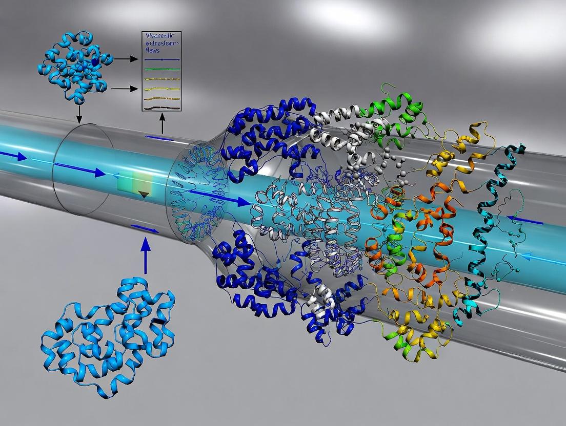
Diagram: 3D FEM for Viscoelastic Extrusion Workflow

3D FEM Workflow for Viscoelastic Extrusion

The Scientist's Toolkit: Key Research Reagent Solutions & Materials

Table 2: Essential Materials for Viscoelastic Polymer Melt Characterization

Item	Function in Research	Example/Notes
Standard Reference Materials	Calibrate rheometers and validate experimental protocols. Provide known rheological properties.	NIST Polyethylene SRM 2490 (for melt viscosity).
Thermally Stable Polymers	Model systems for fundamental studies, minimizing degradation during long tests.	Polystyrene (narrow MWD), Polyethylene, Polypropylene.
Antioxidant Additives	Prevent oxidative degradation of polymer melts during high-temperature testing.	Irganox 1010, BHT. Added at ~0.1 wt%.
Silicone Oil or Inert Gas Blanket	Creates an oxygen-free environment in the rheometer to prevent degradation.	Applied around sample edges or as a purge gas.
Partitioned Plate Geometries	Minimize edge fracture during large deformation tests (e.g., extensional rheometry).	Sentmanat Extensional Rheometry (SER) fixtures.
High-Temperature Grease	Seal gaps in fixtures to prevent sample leakage.	Silicon-based grease stable >250°C.
Solvents for Cleaning	Thoroughly remove polymer residue from rheometer tools after testing.	Xylene (for polyolefins), DCM (for polystyrene).
Non-Newtonian Fluid Standards	Verify shear-thinning and viscoelastic calculations in CFD/FEM software.	Aqueous polyacrylamide or polyvinylpyrrolidone solutions.

The Critical Role of Extrusion in Pharmaceutical Manufacturing (HME, 3D Printing)

Extrusion technologies, specifically Hot-Melt Extrusion (HME) and its integration with 3D Printing (Fused Deposition Modeling), are transformative for pharmaceutical manufacturing. They enable the production of amorphous solid dispersions, controlled-release formulations, and personalized dosage forms. This document details application notes and experimental protocols, framed within a research thesis utilizing 3D finite element modeling (FEM) to simulate viscoelastic polymer melt flow during extrusion, aiming to optimize process parameters and predict product performance.

Table 1: Key Material Properties for HME & Pharmaceutical 3D Printing

Material/Polymer	Tg (°C)	Melt Temp (°C)	Typical Drug Load (%)	Solubility Parameter (MPa^1/2)	Key Application
Soluplus	70	70-80	10-40	~21.1	Amorphous dispersions
Eudragit E PO	48	50-60	10-50	~20.3	Taste masking, immediate release
PVA (Filament)	85	190-220	1-10	~25.8	FDM 3D printing of tablets
PLGA	45-55	N/A (Extruded)	10-70	~21.9	Long-acting implantables
HPMC (HPMCAS)	120	N/A (Thermally processed)	10-30	~23.4	Enteric coatings, stability

Table 2: Impact of Key Extrusion Parameters on Critical Quality Attributes (CQAs)

Process Parameter	Typical Range (HME)	Typical Range (FDM)	Primary Influence on CQA	FEM Modeling Variable
Barrel Temperature	80-180°C	160-250°C (Nozzle)	Drug degradation, Amorphicity	Thermal boundary condition
Screw Speed	50-500 rpm	N/A	Residence time, Shear stress	Rotational velocity, Shear rate
Feed Rate	0.2-5 kg/hr	0.5-2 mm/s (Flow)	Mixing homogeneity, Porosity	Mass inflow rate
Die Diameter	2-5 mm	0.2-0.8 mm (Nozzle)	Die swell, Melt pressure	Geometry, Exit boundary condition
Cooling Rate	10-50°C/s (Calender)	N/A	Crystallinity, Stability	Heat transfer coefficient

Experimental Protocols

Protocol 3.1: Hot-Melt Extrusion for Amorphous Solid Dispersion

Objective: To manufacture an ASD of itraconazole using Soluplus via twin-screw HME. Materials: Itraconazole (API), Soluplus (carrier), co-rotating twin-screw extruder, differential scanning calorimeter (DSC), X-ray powder diffractometer (XRPD). Method:

• Pre-blending: Geometrically mix itraconazole and Soluplus (30:70 w/w) in a turbula mixer for 15 min.
• Extrusion: Feed pre-blend into extruder at 2 kg/hr. Set barrel temperature profile from feed to die: 130/140/150/155°C. Maintain screw speed at 200 rpm.
• Processing: Collect the molten strand, cool on a conveyor belt at 20°C, and pelletize.
• Analysis: Assess amorphicity by DSC (heating rate 10°C/min) and XRPD (5-40° 2θ range). FEM Context: Model this flow to correlate shear rate (from screw speed) with mixing efficiency and predict temperature homogeneity using viscoelastic (Oldroyd-B) constitutive equations.

Protocol 3.2: Fabrication of Personalized Printlets via FDM 3D Printing

Objective: To produce immediate-release printlets using a drug-loaded PVA filament. Materials: HME-produced PVA/paracetamol filament (5% drug load), desktop FDM 3D printer, slicing software, USP dissolution apparatus II. Method:

• Filament Preparation: Manufacture filament per Protocol 3.1 using a single-screw strand extruder and PVA with API.
• Design & Slicing: Design a 10mm diameter, 3mm height tablet (approx. 500 mg) in CAD. Export as STL, slice with 100% infill, 0.2mm layer height, and a rectilinear pattern.
• Printing: Load filament, set nozzle temp to 200°C, bed temp to 60°C, and printing speed to 30 mm/s. Execute print.
• Dissolution Testing: Test printlet in 900 mL pH 6.8 phosphate buffer at 37°C, 50 rpm paddle speed. Sample at 5, 10, 15, 30, 45, 60 min. FEM Context: Model the non-Newtonian, viscoelastic flow through the FDM nozzle to understand shear-thinning behavior and predict strand deposition accuracy for dimensional fidelity.

Visualizations

Diagram Title: HME to FDM Pharmaceutical Manufacturing Workflow

Diagram Title: 3D FEM for Extrusion Process Modeling

The Scientist's Toolkit: Research Reagent Solutions

Table 3: Essential Materials for HME & Pharmaceutical 3D Printing Research

Item	Function/Application	Example Brand/Type
Polymeric Carriers	Form matrix for amorphous solid dispersions; govern release profile.	Soluplus, Eudragit series, PVA, PLGA, HPMCAS
Plasticizers	Lower polymer Tg and melt viscosity, enabling processing at lower temps.	Triethyl citrate, Polyethylene glycol (PEG), Dibutyl sebacate
Melt Flow Index Tester	Empirically measures polymer melt viscosity under standardized conditions.	Key capillary rheometer data feeds FEM model validation.
Twin-Screw Extruder (Lab-scale)	Provides scalable, continuous mixing and conveying of API-polymer blends.	11mm or 16mm co-rotating twin-screw extruder.
Desktop FDM 3D Printer (Pharma-modified)	Enables small-batch, on-demand printing of complex dosage forms.	Printer with enclosed chamber, precision temperature control.
Hot-Stage Microscopy	Visually observes API melting and dissolution into polymer in real-time.	Crucial for initial screening of API-polymer miscibility.
Rheometer (Rotational & Capillary)	Characterizes viscoelastic melt properties for constitutive model input.	Data (G', G'', complex viscosity) essential for accurate FEM.
Stability Chamber	Assesses physical stability (recrystallization) of ASDs under ICH conditions.	Critical for confirming predicted performance from models.

Core FEM Concepts in Fluid Dynamics

The Finite Element Method provides a robust framework for approximating solutions to complex systems of partial differential equations governing fluid flow. For viscoelastic extrusion flows, the method discretizes the domain into finite elements, transforming the continuous problem into a solvable algebraic system.

Key Governing Equations for Viscoelastic Flow:

• Conservation of Mass (Continuity): ∇·u = 0
• Conservation of Momentum: ρ(∂u/∂t + u·∇u) = -∇p + ∇·τ + f
• Constitutive Equation (e.g., Oldroyd-B): τ + λ₁ τ∇ = 2η₀ (D + λ₂ D∇)

Where u is velocity, p is pressure, τ is the extra-stress tensor, D is the rate-of-deformation tensor, ρ is density, η₀ is zero-shear viscosity, λ₁ is relaxation time, and λ₂ is retardation time.

Application Notes for Viscoelastic Extrusion Modeling

Model Formulation and Challenges

Modeling viscoelastic extrusion flows in 3D presents specific challenges addressed by FEM:

• High Weissenberg Number Problem (HWNP): Numerical instabilities as elasticity (Weissenberg number, Wi) increases. Stabilized formulations (SUPG, GLS) are essential.
• Mixed Formulations: Velocity, pressure, and stress fields require inf-sup stable element pairs (e.g., Taylor-Hood elements for velocity-pressure).
• Free Surface Tracking: The extrudate swell interface requires techniques like the Arbitrary Lagrangian-Eulerian (ALE) method or Level Set approaches.

Table 1: Common Constitutive Models for Polymer Extrusion

Model	Equation (Differential Form)	Parameters	Typical Application
Upper-Convected Maxwell (UCM)	τ + λ₁ τ∇ = 2η₀ D	λ₁, η₀	Benchmark, highly elastic melts
Oldroyd-B	τ + λ₁ τ∇ = 2η₀ (D + λ₂ D∇)	λ₁, λ₂, η₀	Boger fluids, solvent-polymer mix
Giesekus	τ + λ₁ τ∇ + (αλ₁/η₀) τ·τ = 2η₀ D	λ₁, η₀, α (mobility)	Shear-thinning polymers
Phan-Thien–Tanner (PTT)	Y(tr(τ))τ + λ₁ τ∇ = 2η₀ D	λ₁, η₀, ε, ξ	Broad range of polymer melts

Table 2: Comparison of Stabilization Techniques for HWNP

Technique	Mechanism	Added Term	Pros	Cons
Streamline-Upwind/Petrov-Galerkin (SUPG)	Adds diffusion along streamlines	τ_SUPG(u·∇δu)·R	Effective for convection dominance	Can over-diffuse stress
Galerkin/Least-Squares (GLS)	Minimizes residual in least-squares sense	τ_GLS L(δu)·R	More robust for mixed problems	Higher computational cost
Log-Conformation Representation (LCR)	Reformulates constitutive equation	Solves for log(τ) instead of τ	Extremely stable at high Wi	Complex implementation

Experimental Protocols for Validation

Protocol: Numerical Simulation of Axisymmetric Die Swell

Aim: To simulate the viscoelastic extrudate swell from a cylindrical die and compare swell ratio with experimental/theoretical data. Materials: FEM software (e.g., COMSOL, ANSYS Polyflow, or open-source FEniCS), high-performance computing cluster. Methodology:

• Geometry & Mesh: Create a 2D axisymmetric domain comprising the die channel (length L=10R) and a large exterior region for the swell. Use a refined, boundary-fitted mesh with high density at the die exit and free surface.
• Physics Setup:
  • Select a viscoelastic constitutive model (e.g., Oldroyd-B).
  • Apply a fully-developed velocity profile (Poiseuille) at the inlet.
  • Set zero traction (neutral) at the outlet.
  • Apply no-slip condition on die walls.
  • Define the free surface using an ALE moving mesh with surface tension.
• Solver Configuration:
  • Use a segregated solver: solve flow field (u-p), then stress field.
  • Implement a GLS stabilization scheme.
  • Employ an adaptive time-stepping scheme, starting with a small time step.
• Analysis: Calculate the steady-state swell ratio (final extrudate radius / die radius) as a function of the Weissenberg number (Wi = λ₁ * U_avg / R).

Protocol: 3D Simulation of Square-Die Extrusion with Corner Vortices

Aim: To capture secondary flows and corner vortex patterns in the extrusion of a viscoelastic fluid through a square cross-section die. Methodology:

• 3D Geometry: Model the die with a square cross-section and sufficient entry length.
• Mesh: Utilize hexahedral elements with local refinement near the corners and walls.
• Boundary Conditions: As per Protocol 3.1, but with a 3D parabolic inlet profile.
• Solver: Use a parallelized coupled solver for efficiency. The log-conformation formulation is recommended for stability.
• Post-Processing: Visualize and quantify the intensity of the secondary flow vectors in the cross-sectional plane and the development of corner vortices along the die length.

Visualization: Workflows and Relationships

Title: FEM Workflow for Viscoelastic Flow Analysis

Title: From Material Parameters to Solver Strategy

The Scientist's Toolkit: Research Reagent Solutions & Essential Materials

Table 3: Key Components for 3D FEM Viscoelastic Extrusion Research

Item / "Reagent"	Function in the Research Context
High-Fidelity Constitutive Model (e.g., PTT, Giesekus)	Defines the mathematical relationship between stress, strain, and strain rate for the viscoelastic fluid. Crucial for accurate physics.
Stabilization Scheme (SUPG, GLS, LCR)	"Stabilizing agent" against numerical instability (HWNP). Allows solutions at practically relevant high Weissenberg numbers.
Mixed Finite Element Formulation (e.g., P2-P1 for u-p)	The core "reaction vessel." Ensures compatibility between interpolation spaces for velocity and pressure, preventing spurious oscillations.
Adaptive Mesh Refinement (AMR) Algorithm	Dynamically concentrates computational elements in regions of high stress gradient (e.g., die lip, corner vortices), optimizing accuracy vs. cost.
Arbitrary Lagrangian-Eulerian (ALE) Framework	Enables tracking of the moving free surface (extrudate swell) by dynamically updating the mesh.
Parallelized Iterative Solver (e.g., GMRES, CG)	Handles the large, sparse, non-linear algebraic systems generated by 3D models efficiently on HPC clusters.
Benchmark Validation Data	Experimental or highly resolved numerical data for canonical flows (e.g., swell ratio, entry pressure drop). Serves as the "calibration standard."

Governing Equations for Viscoelastic Flow

The 3D finite element modeling of viscoelastic extrusion flows is governed by a coupled set of conservation laws and constitutive equations. These form the core mathematical framework for simulating polymer melt or solution behavior during processes relevant to pharmaceutical extrusion, such as hot-melt extrusion for amorphous solid dispersions.

Conservation Laws

These universal laws describe the physical principles of mass, momentum, and energy conservation.

Conservation of Mass (Continuity Equation): [ \nabla \cdot \mathbf{v} = 0 ] Applicability: Assumes incompressible flow, valid for most polymer melts under processing conditions.

Conservation of Momentum (Cauchy Momentum Equation): [ \rho \left( \frac{\partial \mathbf{v}}{\partial t} + \mathbf{v} \cdot \nabla \mathbf{v} \right) = \nabla \cdot \mathbf{\sigma} + \mathbf{f}b ] where the total stress (\mathbf{\sigma}) is decomposed as: [ \mathbf{\sigma} = -p\mathbf{I} + \mathbf{\tau}s + \mathbf{\tau}_p ]

Conservation of Energy: [ \rho C_p \left( \frac{\partial T}{\partial t} + \mathbf{v} \cdot \nabla T \right) = k \nabla^2 T + \mathbf{\tau} : \nabla \mathbf{v} + \dot{Q} ] Critical for modeling thermal effects in hot-melt extrusion of heat-sensitive APIs.

Constitutive Models

Constitutive models relate the polymeric stress ((\mathbf{\tau}_p)) to the deformation history of the fluid. They are required to close the system of equations.

Table 1: Key Differential Constitutive Models for Viscoelastic Fluids

Model	Constitutive Equation	Key Parameters	Typical Application in Pharma Extrusion
Oldroyd-B	( \mathbf{\tau}p + \lambda1 \overset{\triangledown}{\mathbf{\tau}p} = \etap (\dot{\gamma} + \lambda_2 \overset{\triangledown}{\dot{\gamma}}))	(\lambda1): Relaxation time(\lambda2): Retardation time ((\leq \lambda1))(\etap): Polymeric viscosity	Baseline model for constant viscosity Boger fluids; useful for initial stability studies of simple extrudate swell.
Giesekus	( \mathbf{\tau}p + \lambda1 \overset{\triangledown}{\mathbf{\tau}p} + \frac{\alpha \lambda1}{\etap} \mathbf{\tau}p \cdot \mathbf{\tau}p = \etap \dot{\gamma} )	(\lambda1): Relaxation time(\etap): Zero-shear viscosity(\alpha): "Mobility" parameter (0 to 1)	Predicts shear-thinning and normal stresses; models concentrated polymer solutions/melts in die flow.
Phan-Thien–Tanner (PTT)	( Y(tr(\mathbf{\tau}p))\mathbf{\tau}p + \lambda1 \overset{\triangledown}{\mathbf{\tau}p} = \etap \dot{\gamma} )(Y = 1 + \frac{\epsilon \lambda1}{\etap} tr(\mathbf{\tau}p))	(\lambda1): Relaxation time(\etap): Zero-shear viscosity(\epsilon): Extensibility parameter	Captures shear/thinning and extensional viscosity saturation; relevant for flow through contractions.

Note: (\overset{\triangledown}{(\cdot)}) denotes the upper-convected derivative, accounting for frame invariance in flowing polymers: (\overset{\triangledown}{\mathbf{A}} = \frac{\partial \mathbf{A}}{\partial t} + \mathbf{v} \cdot \nabla \mathbf{A} - (\nabla \mathbf{v})^T \cdot \mathbf{A} - \mathbf{A} \cdot (\nabla \mathbf{v})).

Table 2: Quantitative Parameters for Common Pharmaceutical Polymers (Representative)

Polymer (API Carrier)	Model	Typical (\eta_p) [Pa·s] (at 150-180°C)	Typical (\lambda_1) [s]	Critical Parameters	Source (Recent)
HPMCAS (AQOAT)	Giesekus/PTT	(10^3 - 10^4)	(0.01 - 0.1)	(\alpha \approx 0.1-0.3); Strong T-dependence	Drug Dev Ind Pharm, 2023
PVP-VA (Kollidon VA64)	Giesekus	(10^2 - 10^3)	(0.001 - 0.01)	(\alpha \approx 0.15); Pronounced shear-thinning	Int J Pharm, 2022
Soluplus	PTT	(10^4 - 10^5)	(0.1 - 1.0)	High (\epsilon); Significant elastic recoil	J Pharm Sci, 2024
EC (Ethyl Cellulose)	Oldroyd-B/Giesekus	(10^4 - 10^5)	(0.05 - 0.5)	(\lambda2/\lambda1 \approx 0.01)	AAPS PharmSciTech, 2023

Finite Element Implementation Protocol

Protocol 1: Weak Formulation and Galerkin Discretization

Objective: Transform governing equations into a solvable weak form for the Finite Element Method (FEM).

• Problem Domain: Define the 3D extrusion geometry (e.g., screw channel, die).
• Variable Definition: Primary variables: Velocity ((\mathbf{v})), Pressure ((p)), and Polymeric Stress ((\mathbf{\tau}_p)). Temperature ((T)) is coupled for non-isothermal flows.
• Weak Form Development:
  • Multiply momentum equation by test function (\mathbf{w}) and integrate over domain (\Omega): [ \int{\Omega} \mathbf{w} \cdot \rho \frac{D\mathbf{v}}{Dt} \, d\Omega + \int{\Omega} \nabla \mathbf{w} : (-p\mathbf{I} + \mathbf{\tau}s + \mathbf{\tau}p) \, d\Omega = \int{\Gamma} \mathbf{w} \cdot \mathbf{t} \, d\Gamma ]
  • Multiply continuity by test function (q): (\int{\Omega} q (\nabla \cdot \mathbf{v}) \, d\Omega = 0).
  • The constitutive equation for (\mathbf{\tau}_p) is typically solved using the Discrete Elastic-Viscous Split Stress (DEVSS) method to enhance stability, introducing an auxiliary variable.
• Element Choice: Use mixed finite elements (e.g., Taylor-Hood): Quadratic elements for velocity, linear for pressure. The log-conformation representation is recommended for stress to improve high-Weissenberg number convergence.
• Solver Setup: Implement a coupled or sequential iterative solver (Newton-Raphson/Picard). Use adaptive meshing near die walls and corners.

Protocol 2: Experimental Validation via Capillary Rheometry

Objective: Obtain material parameters for constitutive models and validate FEM predictions.

• Material Preparation: Dry polymer (e.g., PVP-VA) and API (e.g., Itraconazole) at 50°C under vacuum for 12h. Physically mix at desired ratio (e.g., 70:30 polymer:API).
• Rheological Characterization:
  • Use a capillary rheometer with a series of dies (L/D ratios: 5, 10, 20, 30).
  • Conduct steady-shear tests at the target extrusion temperature (e.g., 160°C) over a wall shear rate range of (1 - 1000 \, s^{-1}).
  • Record pressure drop ((\Delta P)) and extrudate swell ratio ((d/D)).
  • Perform Bagley correction to obtain true wall shear stress and Rabinowitsch correction for non-Newtonian shear rate.
• Parameter Fitting:
  • Fit shear viscosity data (\eta(\dot{\gamma})) to the Giesekus model function derived from steady shear: [ \eta = \frac{\etap}{[1 + (2\alpha -1)\xi] + \sqrt{1+2\xi}}; \quad \xi = (1-\alpha)\alpha (\lambda1 \dot{\gamma})^2 ]
  • Use first normal stress difference ((N1)) data to independently estimate (\lambda1).
  • Optimize parameters ((\etap, \lambda1, \alpha)) using nonlinear regression (e.g., Levenberg-Marquardt algorithm).
• Validation: Run a 3D FEM simulation of the capillary die flow using the fitted parameters. Compare simulated pressure drop and extrudate swell profile (via particle tracking/interface capture) with experimental results. Iterate on model/parameters until error <15%.

Visualization of Workflows

Title: FEM Workflow for Viscoelastic Extrusion Modeling

Title: Mathematical Framework for Viscoelastic Flow

The Scientist's Toolkit: Research Reagent Solutions & Essential Materials

Table 3: Essential Materials for Viscoelastic Extrusion Modeling & Validation

Item/Category	Function & Relevance	Example/Specification
Model Polymer Systems	Well-characterized, pharmaceutical-grade carriers for method development. Provide benchmark data.	HPMCAS (AQOAT grades), PVP/VA (Kollidon VA64), Soluplus (BASF), Ethyl Cellulose (Standard).
Rheological Additives	Modify viscoelastic response to test model robustness (e.g., tune relaxation time).	Plasticizers (Triethyl citrate, PEG), Flow aids (SiO₂), Chain extenders.
Capillary Rheometer	Primary device for obtaining shear viscosity, normal stress, and extrudate swell data under processing conditions.	Equipped with dual bore (for Bagley correction), laser die swell sensor, and pressure transducers.
Rheometry Software	For fitting constitutive model parameters from experimental flow curves.	TA Instruments TRIOS, Anton Paar RheoCompass with advanced model fitting modules.
High-Performance Computing (HPC) Cluster	Solves large 3D viscoelastic FEM problems with coupled physics.	Multi-core CPUs (≥ 32 cores) with high RAM (≥ 128 GB) or GPU-accelerated solvers (NVIDIA CUDA).
FEM Software	Platform for implementing governing equations and solving boundary value problems.	Commercial: COMSOL Multiphysics, ANSYS Polyflow. Open-Source: FEniCS, OpenFOAM (with viscoelastic solvers).
3D Scanner/High-Speed Camera	Quantifies extrudate swell geometry dynamically for validation.	Laser micrometer or digital image correlation (DIC) system for precise diameter measurement.

Application Notes

In the context of 3D finite element modeling (FEM) for viscoelastic extrusion flows in pharmaceutical development, accurately capturing complex conduit geometries is paramount for predicting drug product properties. The primary challenge lies in the significant computational and methodological disparity between simplified 2D axisymmetric models and full 3D representations of real-world geometries, such as multi-lumen extrusion dies, stent coating applicators, or microfluidic mixers. These 3D features—including non-circular channels, sharp corners, bifurcations, and wall irregularities—introduce secondary flows, asymmetrical stress distributions, and complex free surface deformations that 2D models inherently miss.

The following table summarizes the quantitative impact of moving from 2D to 3D modeling on key viscoelastic flow parameters, based on current research:

Table 1: Quantitative Comparison of 2D vs. 3D Model Predictions for Viscoelastic Extrusion

Parameter	2D Axisymmetric Model Prediction	Full 3D Model Prediction	Discrepancy & Implication
Extrudate Swell Ratio	1.2 - 1.5	1.4 - 2.1 (shape-dependent)	Up to 40% under-prediction in 2D for square/rectangular dies. Critical for dosage form sizing.
Max. Wall Shear Stress (kPa)	120 ± 15	85 - 310 (corner/edge effects)	2D models smooth extremes. 3D reveals stress concentrators causing protein shear denaturation.
First Normal Stress Difference (N1) at Die Exit (kPa)	45 ± 5	Spatially heterogeneous (25 - 70)	2D assumes uniformity. 3D shows lateral gradients affecting film coating uniformity.
Pressure Drop (MPa)	8.5	9.8 - 12.5	2D underestimates by 15-50% for complex geometries, affecting pump sizing and process energy.
Residence Time Distribution Width (s)	2.1	3.8	2D under-represents stagnation in corners, crucial for predicting hot-spots in reactive biopolymer flows.

These discrepancies necessitate rigorous protocols for 3D model validation and application to ensure predictive accuracy in drug process development.

Experimental Protocols

Protocol 1: Micro-Particle Image Velocimetry (μ-PIV) for 3D Flow Field Validation

Objective: To experimentally capture the three-dimensional velocity field of a viscoelastic polymer solution (e.g., 0.1% Polyacrylamide in water/glycerol) within a transparent, scaled extrusion die geometry. Materials: See "Scientist's Toolkit" below. Procedure:

• Fabrication: Manufacture a precision transparent die replica (e.g., of a rectangular or trilobal channel) using stereolithography (SLA) 3D printing with a clear resin. Polish internal surfaces to optical clarity.
• Seeding: Dope the test viscoelastic fluid with fluorescent tracer particles (1 µm diameter, ~1.01 g/cm³ density) at a dilute concentration (~0.01% w/w).
• System Setup: Mount the die replica in a closed-loop flow system with a precision syringe pump. Align a dual-pulsed Nd:YAG laser sheet to illuminate a specific plane within the die (e.g., mid-plane, near-wall plane).
• Image Acquisition: For each flow rate (shear rate from 1 to 100 s⁻¹), capture image pairs at the desired plane using a scientific CMOS camera synchronized with the laser pulses. Repeat for multiple optical planes (z-stack) to reconstruct 3D flow.
• Data Processing: Use cross-correlation algorithms (e.g., in DaVis, MATLAB) to compute the 2D velocity vector field for each plane. Assemble planes to create a 3D velocity map. Compare directly to the velocity field predicted by the 3D FEM simulation at identical planes.

Protocol 2: Flow-Induced Birefringence (FIB) for Stress Field Mapping

Objective: To qualitatively and quantitatively map the principal stress fields within a flowing viscoelastic melt, validating the 3D FEM-predicted stress topology. Procedure:

• Optical Calibration: Place a calibration sample (photoelastic material under known stress) between crossed polarizers to establish the stress-optic coefficient.
• Flow Cell Design: Use a geometrically identical, but optically accessible, flow cell with high-quality glass windows. Ensure minimal mechanical birefringence from the windows.
• Flow Experiment: Pump the transparent viscoelastic melt (e.g., Polystyrene dissolved in oligomeric styrene) through the cell under isothermal conditions.
• Polariscopy: Illuminate the flow cell with a monochromatic light source through a polarizer. Capture the transmitted light through a second, crossed polarizer (analyzer) with a high-resolution camera.
• Analysis: The resulting fringe patterns are contours of constant principal stress difference. Use spectral analysis or phase-stepping methods to quantify the fringe order. Compare the fringe pattern topology (location of fringe concentration, gradients) to the simulated stress fields from the 3D model.

The Scientist's Toolkit: Research Reagent Solutions

Table 2: Essential Materials for 3D Viscoelastic Flow Characterization

Item	Function in Research
Giesekus or Oldroyd-B Model Fluids (e.g., Polyisobutylene in Tetradecane)	Well-characterized, non-Newtonian test fluids with known relaxation times and shear/extensional properties for benchmark model validation.
Fluorescent Polystyrene Microspheres (1 µm)	Tracer particles for μ-PIV; their surface chemistry and density can be matched to the carrier fluid to minimize slip and settling.
Optically Clear SLA Resin (e.g., Formlabs Clear V4)	For rapid, high-resolution prototyping of complex micro-flow geometries for visualization experiments.
Rheometer with Cone-Plate & Capillary Dies	Essential for measuring steady and transient shear viscosity, first normal stress difference, and extensional viscosity—the critical input data for the constitutive model in FEM.
High-Performance Computing (HPC) Cluster License	Enables solving large 3D viscoelastic flow problems (often >10 million degrees of freedom) with coupled thermal and free surface effects in a feasible time.
OpenFOAM with viscoelasticSolvers	Open-source CFD toolbox offering specialized solvers (e.g., pimpleFoam with log-conformation tensor treatment) for stable viscoelastic flow simulations at high Deborah numbers.

Visualization Diagrams

Title: 2D vs 3D Modeling Decision Workflow

Title: μ-PIV Validation Protocol Flowchart

Building and Applying Your 3D Viscoelastic Extrusion FEM Model: A Step-by-Step Guide

Within a broader thesis on 3D Finite Element Modeling (FEM) for viscoelastic extrusion flows in pharmaceutical research, the pre-processing stage is foundational. This stage governs the accuracy, stability, and predictive capability of simulations used to design drug delivery systems, optimize hot-melt extrusion processes, and understand complex non-Newtonian flow behavior. This document outlines application notes and detailed protocols for geometry creation, meshing, and boundary condition definition specific to viscoelastic extrusion flows.

Geometry Creation for Extrusion Flows

The geometry must accurately represent the flow domain, typically from a reservoir, through a complex die (e.g., rod, slit, or co-extrusion), to the free surface (extrudate swell). For 3D modeling, a parametric Computer-Aided Design (CAD) approach is essential.

Protocol: Parametric Die Geometry Construction

• Objective: Create a flexible, watertight 3D CAD model of an extrusion die.
• Software: Utilize parametric CAD tools (e.g., ANSYS DesignModeler, SOLIDWORKS, FreeCAD).
• Steps:
  • Define key parameters as variables: Reservoir diameter (D_res), die land length (L_land), die gap height (H_gap), and die entrance angle (α).
  • Sketch the 2D axisymmetric profile or full 3D cross-section.
  • Revolve (for axisymmetric) or extrude (for 3D) the sketch to create the solid flow volume.
  • Use a "Boolean Subtract" operation to remove the die walls, leaving only the fluid domain volume.
  • Apply fillets to sharp corners (e.g., at the entrance) to avoid singularities in stress calculations, with a recommended radius of 5-10% of H_gap.
• Key Consideration: The geometry should be "clean" (no stray edges, gaps) to prevent meshing failures.

Table 1: Typical Geometric Parameters for Pharmaceutical Extrusion Die Modeling

Parameter	Symbol	Typical Range	Common Value (Example)	Function
Reservoir Diameter	D_res	5 - 20 mm	10 mm	Provides initial flow development zone.
Die Land Length	L_land	(5 - 20) × H_gap	10 mm	Dominant region for shear flow and pressure drop.
Die Gap Height	H_gap	0.5 - 3 mm	1 mm	Defines the final product dimension and shear rate.
Entrance Angle	α	30° - 90°	45°	Controls the extensional flow strength and vortex formation.
Corner Fillet Radius	R_fillet	(0.05 - 0.1) × H_gap	0.1 mm	Reduces stress singularities, improves convergence.

Meshing Strategies for Viscoelastic Flows

Meshing for viscoelastic fluids (e.g., polymer melts, gel-based formulations) is critical due to steep stress boundary layers and potential stress singularities.

Protocol: Boundary Layer Meshing for the Die Wall

• Objective: Resolve the high stress gradient near the die wall.
• Method: Structured or hybrid meshing with inflation layers.
  • Define the die wall as the boundary for inflation.
  • Specify the first layer thickness (δ) based on the estimated viscoelastic stress boundary layer thickness. A rule of thumb: δ ≈ 0.01 * H_gap.
  • Set a growth rate between 1.1 and 1.2.
  • Use 10-15 inflation layers for a Giesekus or Phan-Thien–Tanner model.
• Validation: Perform a mesh sensitivity study, monitoring the wall shear stress and normal stress difference at the die exit.

Table 2: Mesh Sensitivity Study Results for a Giesekus Fluid (η₀=1000 Pa·s, λ=1 s)

Mesh Case	Total Elements	Min Element Size (mm)	Wall Shear Stress (kPa)	Extrudate Swell Ratio	Relative Error (Swell)
Coarse	85,000	0.05	121.5	1.15	8.7%
Medium	320,000	0.02	132.1	1.23	2.4%
Fine	1,200,000	0.008	135.3	1.26	Reference
Very Fine	4,500,000	0.003	135.6	1.26	0.0%

Protocol: Free Surface (Extrudate Swell) Mesh Adaptation

• Objective: Capture the moving interface where the fluid exits the die.
• Method: Use an Arbitrary Lagrangian-Eulerian (ALE) or Volume-of-Fluid (VOF) technique with mesh smoothing/remeshing.
  • Extrude the initial mesh beyond the die exit to create an air/vacuum domain.
  • Define the interface as a moving boundary.
  • Enable mesh smoothing to prevent excessive distortion.
  • Set convergence criteria for the swell shape (e.g., change in swell ratio < 0.1% between iterations).

Boundary Condition Definition

Accurate boundary conditions (BCs) are vital for realistic simulation of the extrusion process.

Protocol: Setting Up Flow and Stress BCs

• Inlet: Apply a fully-developed velocity profile (e.g., parabolic for Newtonian, computed profile for viscoelastic) or a prescribed flow rate (Q). Stress components should be consistent with the constitutive model.
• Die Walls: Apply the no-slip condition (u=0). For highly viscous melts, wall slip can be modeled using a Navier slip law if experimental data is available.
• Outlet/Extrudate Surface: Define atmospheric pressure (p=0 gauge) at the far outlet. For the free surface, apply a zero-traction condition and specify surface tension coefficient (γ) if significant.
• Symmetry Planes: Utilize symmetry BCs to reduce model size where applicable (u_n=0, τ_t=0).

Table 3: Common Boundary Conditions for Extrusion Flow FEM

Boundary	Velocity/Pressure Condition	Stress Condition	Notes
Inlet	u_z = f(r), Q specified	τ_rr, τ_rz from profile	Use a "development length" before the die.
Die Wall	u = 0 (No-slip)	---	Critical for shear rate calculation.
Symmetry Axis	u_r = 0, ∂u_z/∂r = 0	τ_rz = 0	Reduces computational cost.
Free Surface	n · σ · t = 0 (traction)	---	May include surface tension: n · σ = γκ n.
Outlet (far field)	p = 0 (gauge)	---	Should be placed sufficiently downstream.

Workflow and The Scientist's Toolkit

Title: FEM Pre-processing Workflow for Extrusion Modeling

The Scientist's Toolkit: Key Research Reagent Solutions & Materials

Item/Reagent	Function in Research	Example/Specification
Pharmaceutical Polymer Melt	Viscoelastic test fluid.	Hydroxypropyl cellulose (HPC), Ethyl cellulose, API-loaded polymer blends.
Rheometer (Rotational & Capillary)	Characterize η(γ̇), N1, relaxation time (λ).	TA Instruments DHR, Malvern Capillary Rheometer. Fit data to Giesekus/PTT models.
Parametric CAD Software	Create and modify precise die geometries.	ANSYS SpaceClaim, SOLIDWORKS, openSCAD.
FEM Pre-processor	Geometry cleanup, meshing, BC assignment.	ANSYS Meshing, Gmsh (open-source), SALOME.
High-Performance Computing (HPC) Cluster	Run 3D transient viscoelastic simulations.	Multi-core CPUs (64+ cores), High RAM (>256 GB).
Post-processing Software	Visualize flow, stress fields, extrudate shape.	ParaView, ANSYS CFD-Post, MATLAB for data analysis.
Validation Data	Benchmark simulation results.	Laser-based extrudate swell measurement, in-die pressure transducer data.

Within the broader thesis on 3D finite element modeling (FEM) for viscoelastic extrusion flows, accurate material property input is paramount. For pharmaceutical applications like hot-melt extrusion (HME) of amorphous solid dispersions, the rheological characterization of drug-polymer blends governs the model's predictive fidelity. This document details application notes and protocols for characterizing these viscoelastic properties and implementing them into FEM simulations.

Rheological Characterization: Key Data & Protocols

Core Rheological Parameters for FEM Input

Quantitative data from rheological characterization feeds directly into constitutive models (e.g., Generalized Newtonian, Upper-Convected Maxwell) within the FEM solver. Key parameters are summarized below.

Table 1: Essential Rheological Parameters for 3D Viscoelastic FEM

Parameter	Symbol	Unit	Description	Relevance to FEM
Zero-shear viscosity	η₀	Pa·s	Viscosity at near-zero shear rate	Determines baseline flow resistance.
Infinite-shear viscosity	η∞	Pa·s	Viscosity at very high shear rates	Asymptotic value in Carreau-type models.
Power-law index	n	-	Measure of shear-thinning behavior	Key for Ostwald-de Waele (Power Law) model.
Consistency index	K	Pa·sⁿ	Related to fluid thickness in Power Law
Relaxation time	λ	s	Characteristic time for stress decay	Critical for viscoelasticity (Maxwell models).
Elastic modulus	G'	Pa	Storage modulus, solid-like response	Dictates die swell & elastic recoil in extrusion.
Viscous modulus	G"	Pa	Loss modulus, liquid-like response
Glass Transition Temp.	T_g	°C	Polymer/drug blend transition temperature	Sets processing temperature window.

Table 2: Exemplary Rheological Data for Common HME Polymer (PVP VA64) Blends

Drug Load (%)	Temp. (°C)	η₀* (Pa·s)	Power-law index (n)	Relaxation Time λ (s)	G' at 1 rad/s (Pa)
0% (Neat Polymer)	160	1250	0.65	0.12	450
20% Itraconazole	160	4800	0.58	0.25	1200
30% Itraconazole	160	9500	0.52	0.38	2100
20% Felodipine	160	3100	0.61	0.18	850

*Estimated via Carreau model fit at low shear rates.

Detailed Experimental Protocols

Protocol 1: Oscillatory Shear Rheometry for Viscoelastic Properties

Objective: To determine the storage (G') and loss (G") moduli, complex viscosity (η*), and relaxation spectrum of a drug-polymer blend.

Materials & Equipment:

• Parallel-plate rheometer (e.g., TA Instruments DHR, Malvern Kinexus)
• 8-25 mm diameter parallel plates (serrated recommended to prevent slip)
• Hot-melt extruded ribbons or compression-molded disks of drug-polymer blend
• Environmental test chamber for temperature control

Procedure:

• Sample Preparation: For consistent results, prepare samples via small-scale HME. Mill the extrudate and compression mold into 1.0 mm thick disks at temperature (T_g + 30°C) under slight pressure.
• Instrument Setup: Install serrated parallel plates. Set initial gap to 1.5 mm. Preheat to the desired test temperature (e.g., 160°C). Allow thermal equilibrium for 10 min.
• Loading & Trimming: Load the pre-formed disk onto the bottom plate. Lower the top plate to a 1.0 mm measuring gap. Trim excess material carefully.
• Strain Amplitude Sweep: At a fixed angular frequency (ω = 10 rad/s), perform a strain sweep (e.g., 0.01% to 10%) to identify the linear viscoelastic region (LVR).
• Frequency Sweep: Within the LVR (e.g., at 0.5% strain), perform a frequency sweep from 100 to 0.1 rad/s. Record G', G", and η*.
• Data Analysis: Fit the frequency sweep data to a model (e.g., Maxwell or Cross) to extract the zero-shear viscosity (η₀) and mean relaxation time (λ = 1/ω_cross, where G'=G").

Protocol 2: Steady Shear Viscosity for Flow Curve Generation

Objective: To obtain the steady shear viscosity (η) vs. shear rate (γ̇) profile for implementation into Generalized Newtonian models.

Procedure:

• Sample Loading: Follow steps 1-3 from Protocol 1.
• Shear Rate Ramp: Perform a logarithmic shear rate ramp from 0.01 s⁻¹ to 100 s⁻¹ at a constant temperature.
• Corrections: Apply necessary corrections for non-Newtonian flow if required by the rheometer software.
• Model Fitting: Fit the resulting flow curve to the Carreau-Yasuda model: η(γ̇) = η∞ + (η₀ - η∞) * [1 + (λcγ̇)^a]^((n-1)/a), where λc is a time constant and a is a fitting parameter. Extract η₀, η∞, and the power-law index n.

Implementation into 3D Finite Element Modeling

The characterized properties are input into the FEM software (e.g., COMSOL Multiphysics, ANSYS Polyflow) to define the material model for the extrusion flow simulation.

Table 3: Mapping of Experimental Data to FEM Input Parameters

FEM Constitutive Model	Required Experimental Input	Source Protocol
Power Law (Ostwald-de Waele)	Consistency index (K), Power-law index (n)	Protocol 2 (Steady Shear)
Carreau-Yasuda	η₀, η∞, λ_c, n, a	Protocol 2 (Steady Shear)
Upper-Convected Maxwell (UCM)	Zero-shear viscosity (η₀), Relaxation time (λ)	Protocol 1 (η₀ from G"/ω), Protocol 1 (λ from crossover)

Title: From Material Characterization to 3D FEM Simulation Workflow

The Scientist's Toolkit: Key Research Reagent Solutions

Table 4: Essential Materials for Drug-Polymer Rheology Characterization

Item / Reagent	Function & Relevance in Characterization
PVP-VA64 (Copovidone)	Common hydrophilic polymer for amorphous solid dispersions; baseline for studying plasticizing effect of API.
HPMCAS (Hypromellose Acetate Succinate)	Enteric polymer; rheology is highly pH and grade-dependent, important for modeling enteric extrusion.
Soluplus (PVA-PEG graft copolymer)	Low-T_g polymer; exhibits distinct thermo-rheological properties for low-temperature extrusion modeling.
Itraconazole	Model BCS Class II drug; high melting point and low solubility impart significant viscosity increase in blends.
Glycerol Monostearate	Common plasticizer/excipient; used to modulate blend rheology and study its effect on viscoelastic parameters.
Triton X-100 (or similar surfactant)	Added in small amounts to study its effect on melt fracture onset in extrusion, a key simulation validation point.
Antioxidants (e.g., BHT)	Prevent polymer degradation during prolonged rheological testing at high temperatures, ensuring data stability.
Compression Molding Kit	For preparing uniform, bubble-free disks/plaques from extrudate for accurate rheometer loading.

Title: Constitutive Model Selection Based on Experimental Data

Solver Selection and Settings for Steady-State and Transient Viscoelastic Flow

Within the broader thesis on 3D finite element modeling for viscoelastic extrusion flows relevant to pharmaceutical polymer processing, the choice of numerical solver and its parameters is critical. This document provides application notes and protocols for selecting and configuring solvers to accurately model both steady-state and transient viscoelastic flow behavior, which is essential for predicting drug-loaded filament extrusion in applications like 3D printing of solid dosage forms.

Solver Fundamentals & Selection Criteria

Core Equation Systems

Viscoelastic flow is governed by the coupled system of the Cauchy momentum equation and a constitutive equation for the polymer stress. For an incompressible fluid: Conservation of Momentum: ∇·σ + ρg = ρ * Dv/Dt, where σ = -pI + τ + 2ηsD. Constitutive Model (e.g., Oldroyd-B): τ + λ τ∇ = 2ηpD. Here, τ is the polymer stress tensor, λ is relaxation time, ηp and ηs are polymer and solvent viscosities, and D is the rate-of-deformation tensor.

Solver Type Comparison

The high Weissenberg number problem (HWNP) and the elliptic nature of the momentum-constitutive coupling necessitate specialized solvers.

Table 1: Solver Types for Viscoelastic Flow

Solver Type	Description	Best For	Stability Considerations
Coupled (Monolithic)	Solves all variables (u, p, τ) simultaneously.	Transient flows, high accuracy.	High memory, ill-conditioned matrix.
Decoupled (Segregated)	Solves equations sequentially (e.g., EVSS, DEVSS).	Steady-state, complex geometries.	Requires stabilization (e.g., SU, SUPG).
Stabilized Explicit	Explicit treatment of stress equation.	Fast prototyping, moderate We.	Strict time-step limit (CFL condition).
Log-Conformation	Solves for logarithm of conformation tensor.	High Weissenberg number flows.	Mitigates HWNP; complex implementation.

Key Selection Parameters

Selection is based on:

• Flow Type: Steady vs. transient.
• Weissenberg Number (We): We = λ * (characteristic shear rate). Defines flow elasticity.
• Model Complexity: Differential vs. integral constitutive models.
• Computational Resources.

Table 2: Solver Recommendation Matrix

Flow Regime	We Range	Recommended Solver	Critical Settings
Steady, Low We	We < 1	Segregated (EVSS)	SU stabilization, Picard iteration.
Steady, High We	We > 1	Log-Conformation	Newton iteration, direct linear solver (MUMPS).
Transient, Startup	Any	Coupled Implicit	BDF2 time scheme, adaptive time-stepping.
Transient, Oscillatory	Any	Coupled or Segregated	GMRES linear solver, strict convergence tolerance.

Protocols for Solver Configuration

Protocol for Steady-State Analysis using a Decoupled (EVSS) Approach

Aim: Obtain a steady viscoelastic flow field for extrusion die design analysis. Materials: See Scientist's Toolkit. Workflow:

• Mesh Generation: Create a 3D tetrahedral mesh of the flow geometry (e.g., extrusion die). Apply boundary layer refinement near walls.
• Equation Setup: Implement the EVSS-G formulation. Split stress: τ = 2ηp(S + D), where S is an auxiliary variable.
• Boundary Conditions: Set inflow velocity (volumetric flow rate), no-slip walls, and zero-traction outflow.
• Solver Settings:
  • Nonlinear Iteration: Use Picard (fixed-point) iteration for robustness.
  • Stabilization: Enable Streamline-Upwind (SU) for the constitutive equation.
  • Convergence Criteria: Set residual tolerance to 1e-6 for all equations.
  • Relaxation: Apply a stress relaxation factor of 0.7 to aid convergence.
• Initialization: Start from a corresponding Newtonian or lower-We solution.
• Run & Monitor: Increment Weissenberg number stepwise. Monitor the stress components and velocity at key points until they stabilize.

Solver Workflow for Steady-State Viscoelastic Flow

Protocol for Transient Analysis using a Coupled Implicit Solver

Aim: Simulate time-dependent behavior such as extrusion startup or flow instability. Materials: See Scientist's Toolkit. Workflow:

• Initial Condition: Use a quiescent state (zero velocity, stress) or a previously computed steady-state solution.
• Time Scheme: Select a second-order Backward Differentiation Formula (BDF2) for time integration.
• Solver Coupling: Use a fully coupled (monolithic) approach where the system [u, p, τ] is solved simultaneously at each time step.
• Linear Solver Configuration:
  • Use a direct solver (e.g., MUMPS) for accuracy with moderate mesh sizes.
  • For large 3D problems, use a preconditioned Krylov solver (e.g., GMRES with block ILU preconditioner).
• Time-Step Control: Implement adaptive time-stepping based on nonlinear solver convergence behavior. Set initial Δt = 0.1λ.
• Run Simulation: Execute from t=0 to the desired end time. Output field data at intervals for analysis of transient evolution.

Table 3: Typical Transient Solver Parameters (Oldroyd-B Model)

Parameter	Recommended Value	Purpose
Initial Time Step (Δt)	0.1 * λ	Resolves initial transient.
Maximum Time Step	1.0 * λ	Prevents skipping dynamics.
BDF Order	2	Stability & accuracy.
Nonlinear Tol.	1e-5	Balance speed/accuracy.
Absolute Tol. (Stress)	1e-4	Critical for stress components.

Transient Coupled Solver Protocol Diagram

The Scientist's Toolkit: Research Reagent Solutions

Table 4: Essential Computational Tools & "Reagents"

Item	Function in Viscoelastic Flow Simulation	Example/Note
Finite Element Library	Core infrastructure for discretization and assembly.	FEniCS, deal.II, COMSOL Multiphysics.
Linear Solver Suite	Solves the large, sparse linear systems at the heart of the computation.	PETSc, MUMPS, Intel MKL PARDISO.
Constitutive Model Library	Implements viscoelastic stress equations.	Oldroyd-B, Giesekus, PTT, Rolie-Poly.
Mesh Generator	Creates the discretized spatial domain.	Gmsh, ANSYS Meshing, built-in tools.
Stabilization Scheme	Prevents numerical oscillations in advection-dominated stress equation.	SU, SUPG, EVSS/DEVSS, log-conformation.
Post-Processor	Visualizes and quantifies results (stress, velocity, streamlines).	ParaView, VisIt, MATLAB.
High-Performance Computing (HPC) Cluster	Provides necessary CPU/GPU resources for 3D transient simulations.	Linux cluster with MPI support.

This application case study is a component of a broader doctoral thesis investigating advanced 3D finite element modeling (FEM) techniques for viscoelastic extrusion flows. The research aims to develop high-fidelity, coupled thermo-mechanical models that accurately predict the complex distribution of an Active Pharmaceutical Ingredient (API) within a polymer matrix during hot-melt extrusion (HME). This is critical for ensuring content uniformity in amorphous solid dispersions, a key formulation strategy for enhancing the bioavailability of poorly soluble drugs.

Table 1: Typical Material Properties for HME Modeling

Material/Parameter	Typical Value Range	Unit	Function in Model
API (e.g., Itraconazole)	10 - 40	% w/w	Dispersed phase; influences rheology
Polymer (e.g., HPMCAS)	60 - 90	% w/w	Continuous viscoelastic matrix
Melt Density (Polymer-API)	1000 - 1300	kg/m³	Required for momentum equations
Zero-Shear Viscosity (Polymer)	100 - 10,000	Pa·s	Key rheological parameter
Power-Law Index (n)	0.3 - 0.8	-	Shear-thinning behavior
Activation Energy (Ea)	50 - 150	kJ/mol	Temperature-dependent viscosity
Thermal Conductivity (Melt)	0.15 - 0.30	W/(m·K)	Heat transfer calculation
Specific Heat Capacity (Melt)	1500 - 2500	J/(kg·K)	Energy equation

Table 2: Key Output Metrics from 3D FEM API Distribution Simulation

Simulation Output Metric	Definition	Target for Homogeneity	Typical Value from Model
Coefficient of Variation (CoV)	(Standard Deviation / Mean) x 100%	< 5.0%	2.5% - 8.0% (process-dependent)
Residence Time Distribution (RTD) Width	Variance of residence time curve	Minimized for narrow distribution	30 - 120 seconds
Maximum Shear Rate	Peak local shear rate in screw channel	< Critical shear for degradation	100 - 500 s⁻¹
Melt Temperature Range	ΔT across melt pool	Minimized (< 10°C)	5 - 25°C
Dispersive Mixing Index (λ)	Measure of interfacial stretching	Closer to 1.0 indicates better mixing	0.7 - 0.95

Experimental Protocols for Model Validation

Protocol 1: Preparation of Calibration Samples for API Distribution Analysis Objective: To create samples with known API distributions for calibrating and validating the FEM model predictions.

• Materials: API (e.g., Itraconazole), polymer carrier (e.g., HPMCAS), co-rotating twin-screw hot-melt extruder (e.g., 11mm or 18mm diameter), liquid nitrogen.
• Procedure: a. Pre-blend API and polymer in a turbula mixer for 10 minutes at 49 rpm. b. Process the blend through the HME at a predetermined set of parameters (e.g., Barrel Temp: 150°C, Screw Speed: 200 rpm, Feed Rate: 0.5 kg/hr). c. Collect the extrudate strand and rapidly quench in liquid nitrogen to freeze-in the morphology. d. Section the strand transversely and longitudinally using a precision microtome at -20°C to create 100 µm thick slices. e. Analyze API concentration across sections using Raman chemical imaging (e.g., 785 nm laser, 1 µm spatial resolution). Map the relative API peak intensity (e.g., ~1690 cm⁻¹) against the polymer peak.
• Data Analysis: Calculate the experimental Coefficient of Variation (CoV) of API intensity across multiple pixel maps for direct comparison with the FEM-predicted concentration field.

Protocol 2: Rheological Characterization for Model Input Objective: To obtain accurate viscoelastic data for constitutive equations in the FEM solver.

• Materials: Parallel-plate rheometer (e.g., 25 mm diameter), prepared polymer-API blends (identical to HME feed).
• Procedure: a. Load a sample disk between pre-heated plates (gap: 1.0 mm). b. Perform a frequency sweep (e.g., 0.1 to 100 rad/s) at a strain within the linear viscoelastic region (determined via amplitude sweep) at multiple temperatures (e.g., 140, 150, 160°C). c. Conduct steady-state shear rate sweeps (e.g., 0.01 to 100 s⁻¹) at the same temperatures. d. Perform time-temperature superposition (TTS) to create master curves for storage (G') and loss (G'') moduli.
• Data Analysis: Fit the Cross-WLF model or a modified Carreau-Yasuda model to the complex viscosity data. Extract parameters: zero-shear viscosity, power-law index, relaxation time, and activation energy. These are direct inputs for the viscoelastic flow model.

The Scientist's Toolkit: Research Reagent Solutions

Table 3: Essential Materials for HME Modeling & Validation

Item	Function in Research
Co-rotating Twin-Screw Extruder (Lab-scale)	Provides the physical extrusion process for validating simulation results and producing samples. Key parameters: screw diameter, L/D ratio, modular screw design.
Polymer Carrier (e.g., HPMCAS, PVPVA)	Forms the viscoelastic continuous phase. Its rheology dictates flow behavior and is critical for model accuracy.
Model API (e.g., Itraconazole, Felodipine)	Poorly soluble compound used as the dispersed phase. Its distribution is the primary simulation output.
High-Performance Computing (HPC) Cluster	Solves computationally intensive 3D FEM simulations with coupled fluid flow, heat transfer, and species transport.
Computational Fluid Dynamics (CFD) Software	Platform for implementing viscoelastic models (e.g., Phan-Thien-Tanner, Giesekus) and solving governing equations (ANSYS Polyflow, COMSOL).
Rheometer with High-Temperature Cell	Characterizes the temperature- and shear-dependent viscoelastic properties of the melt, providing essential input data for the model.
Raman Chemical Imaging Microscope	Non-destructive, high-resolution mapping of API distribution in quenched extrudate sections for direct model validation.

Visualizations

Title: 3D FEM Workflow for API Distribution in HME

Title: Protocol for Developing & Validating the HME Distribution Model

This application note, framed within a thesis on 3D finite element modeling (FEM) for viscoelastic extrusion flows, details the protocols for simulating printability in extrusion-based 3D bioprinting. Printability—encompassing filament formation, stacking fidelity, and structural integrity—is critically dependent on the viscoelastic behavior of bioinks under extrusion and deposition. High-fidelity FEM simulation provides a predictive tool to optimize bioink formulations and printing parameters before costly experimental trials, accelerating development in tissue engineering and drug screening.

Key Quantitative Parameters for Simulation

The following table summarizes critical input and output parameters for printability simulation, derived from current literature and experimental standards.

Table 1: Key Quantitative Parameters for Printability Simulation

Parameter Category	Specific Parameter	Typical Range / Value	Description & Impact on Printability
Bioink Rheological Properties	Shear Storage Modulus (G')	100 - 10,000 Pa	Dominates at low shear; critical for shape retention.
	Shear Loss Modulus (G")	50 - 5,000 Pa	Dominates during flow; affects extrusion pressure.
	Zero-Shear Viscosity (η₀)	10 - 10^5 Pa·s	Viscosity at rest; influences filament collapse.
	Power Law Index (n)	0.1 - 0.8 (Shear-thinning)	Degree of shear-thinning; eases extrusion but affects post-deposition.
	Yield Stress (τ_y)	10 - 500 Pa	Minimum stress to initiate flow; prevents nozzle dripping.
	Relaxation Time (λ)	0.1 - 10 s	Viscoelastic timescale; affects filament recoil and fusion.
Printing Process Parameters	Nozzle Diameter (D)	100 - 500 μm	Directly impacts shear rate and resolution.
	Printing Speed (U)	1 - 20 mm/s	Affects shear rate and deposition rate.
	Extrusion Pressure / Flow Rate (Q)	1 - 100 μL/min	Governs material deposition volume.
	Layer Height (h)	0.5 - 1.0 * D	Influences inter-layer bonding and stackability.
Simulation Output Metrics	Wall Shear Stress in Nozzle	10^2 - 10^4 Pa	Indicates potential cell damage.
	Extrudate Swell Ratio (d/D)	1.0 - 2.5	Post-extrusion diameter vs. nozzle diameter; affects accuracy.
	Filament Spanning Capability	Max. Span Length (L)	Ability to bridge gaps without sagging.
	Inter-layer Bonding Strength	Simulated Fusion Index	Predicts structural integrity of stacked layers.

Detailed Finite Element Simulation Protocol

This protocol describes the setup for a transient, 3D, non-isothermal simulation of bioink extrusion using a commercial FEM package (e.g., COMSOL Multiphysics or ANSYS Polyflow).

Protocol 1: 3D FEM Simulation of Viscoelastic Extrusion Flow

Objective: To predict the filament morphology, shear stress history, and post-deposition behavior of a viscoelastic bioink during extrusion bioprinting.

Materials (Software):

• FEM software with coupled fluid dynamics and heat transfer modules.
• Viscoelastic constitutive model library (e.g., Giesekus, Oldroyd-B, Cross).
• High-performance computing workstation (≥ 32 GB RAM, multi-core CPU).

Methodology:

• Geometry Creation:
  • Construct a 3D model consisting of: (a) a syringe reservoir, (b) a conical converging section, (c) a straight cylindrical nozzle (length ≥ 10× diameter), and (d) a deposition stage positioned 0.5-1.0 mm from the nozzle exit.
  • Parameterize key dimensions (Nozzle D, Stage Gap) for easy variation.

• Mesh Generation:

  • Apply an extremely fine boundary layer mesh at the nozzle wall to resolve high shear gradients.
  • Use swept meshing for the nozzle. Ensure mesh independence by refining until key outputs (e.g., pressure drop) change by <2%.

• Material Model Definition:

  • Select a viscoelastic constitutive model. The Giesekus model is often suitable for shear-thinning polymer solutions like alginate or hyaluronic acid.
  • Input rheological parameters (from Table 1) obtained from rotational rheometry: η₀, η_∞, λ, and the mobility parameter (α).
  • Define density and specific heat capacity if including thermal effects.

• Boundary Conditions & Physics Setup:

  • Inlet: Apply a volume flow rate (Q) or pressure (P) boundary condition.
  • Walls: Apply no-slip condition. Set wall temperature if simulating thermo-responsive bioinks.
  • Nozzle Outlet & Stage: Apply a "free surface" or "phase field" interface to model the moving air-bioink boundary and filament deposition.
  • Gravity: Include gravitational acceleration in the vertical direction.
  • Moving Mesh: Implement an Arbitrary Lagrangian-Eulerian (ALE) method to handle the deforming geometry of the extruding filament.

• Solver Configuration:

  • Use a segregated or coupled solver with a robust PARDISO direct solver for the linearized steps.
  • Implement a gradual ramp of the inlet flow rate over the initial timesteps to improve convergence.
  • Set a time-dependent study with a step size small enough to capture filament advancement.

• Post-Processing & Analysis:

  • Extract the velocity and stress fields within the nozzle.
  • Calculate the wall shear stress profile along the nozzle length.
  • Visualize the extrudate swell and measure the steady-state filament diameter.
  • Track the deformation and stress relaxation of the deposited filament over time.

Experimental Validation Protocol

Simulation predictions must be validated against physical printing experiments.

Protocol 2: Experimental Validation of Simulated Printability

Objective: To correlate simulated printability metrics (extrudate swell, filament stability) with experimental observations.

Materials:

• Extrusion bioprinter (e.g., BIO X, Regemat3D).
• Bioink (e.g., 3% w/v Alginate, 5 million cells/mL).
• Syringes (3 mL) and conical nozzles (22G-27G).
• High-speed camera mounted on microscope.
• ImageJ software for analysis.

Methodology:

• Filament Morphology Analysis:
  • Print a straight filament onto a stationary substrate using parameters matching the simulation.
  • Capture the extrusion and initial deposition (first 5 seconds) using a high-speed camera (>100 fps).
  • Use ImageJ to measure the filament diameter at multiple points. Calculate the average experimental extrudate swell ratio = (Avg. Filament D) / (Nozzle D).
  • Compare with the simulation-predicted swell ratio.

• Grid Structure Fidelity Test:
  • Simulate the printing of a 10x10 mm, 2-layer grid structure with a defined strand spacing.
  • Perform the actual print with identical parameters.
  • Acquire top-down images of the printed grid.
  • Quantify the pore uniformity and strand diameter consistency. Measure any strand sagging or fusion deviations from the designed model.
  • Qualitatively and quantitatively compare the simulated filament shape and fusion points with the experimental image.

Visualizations

Title: FEM Simulation and Validation Workflow for Bioprinting

Title: From Simulation Inputs to Printability Prediction

The Scientist's Toolkit: Research Reagent Solutions

Table 2: Essential Materials for Bioink Printability Studies

Item	Function/Description	Example Product/Chemical
Base Hydrogel Polymers	Provide the viscoelastic scaffold for cell encapsulation and extrusion.	Sodium Alginate (e.g., Pronova UP MVG), Gelatin Methacryloyl (GelMA), Hyaluronic Acid (e.g., Lifecore).
Crosslinking Agents	Induce gelation to stabilize the printed structure post-extrusion.	Calcium Chloride (for alginate), Photoinitiators (e.g., LAP for GelMA UV crosslinking).
Rheology Modifiers	Fine-tune shear-thinning and yield stress behavior for improved printability.	Nanocellulose (CNC), Gellan Gum, Clay Nanosilicates (Laponite).
Biological Components	Provide the living, functional element for tissue models.	Primary Cells (e.g., HUVECs, MSCs), Cell Culture Media, Growth Factors.
Commercial Bioinks	Pre-formulated, characterized bioinks for standardized testing.	CELLINK Bioink (GelMA-based), Allevi Gelatin-Alginate blends, REGEMAT 3D Bioink.
Support Bath/Medium	A yield-stress fluid to support printing of complex, low-viscosity structures.	Carbopol Microgels, Gelatin Slurry, FRESH (Freeform Reversible Embedding).
FEM Simulation Software	Platform for developing the viscoelastic extrusion flow models.	COMSOL Multiphysics (CFD Module), ANSYS Polyflow, openFOAM.
Rotational Rheometer	Essential for measuring G', G", yield stress, and viscosity to parameterize simulations.	Anton Paar MCR series, TA Instruments Discovery HR.

Solving Convergence Issues and Optimizing 3D Viscoelastic FEM Simulations

Within the broader thesis on 3D finite element modeling for viscoelastic extrusion flows in pharmaceutical manufacturing, the High Weissenberg Number Problem (HWNP) presents a fundamental computational barrier. As the Weissenberg number (Wi)—the ratio of elastic forces to viscous forces—increases, standard numerical schemes for solving constitutive equations (e.g., Oldroyd-B, Giesekus) fail, limiting the simulation of realistic processing conditions for polymeric drug carriers and biogels. This document provides application notes and protocols to identify, diagnose, and overcome HWNP in a research setting.

Key Numerical Instabilities: Identification and Metrics

The onset of HWNP is signaled by specific numerical artifacts. The following table summarizes key indicators and their quantitative thresholds.

Table 1: Diagnostic Indicators of HWNP Onset in 3D FEM Viscoelastic Flow Simulations

Indicator	Description	Typical Pre-Failure Threshold	Measurement Method
Stress Overshoot	Viscoelastic stress exceeds physically realistic values.	Local stress > 10x inlet stress	Monitor log files for max(isotropic pressure) and max(extra stress trace).
Mass Conservation Error	Loss of divergence-free velocity field.	Global mass error > 1%	Calculate ∫ (∇·v) dΩ over domain Ω per time step.
Loss of Positive Definiteness	Loss of positive eigenvalues for conformation tensor.	Minimum eigenvalue < -1e-6	Output min(eig(C)) for each element at each iteration.
Newton Iteration Failure	Solver fails to converge within allotted iterations.	Residual norm > 1e3 & oscillating	Check nonlinear solver log for residual history.
Gradient Blow-up	Spatially unbounded growth of velocity/stress gradients.	‖∇τ‖ > 1e7 at any node	Post-process gradient fields of stress (τ) components.

Core Stabilization Protocols

Detailed methodologies for implementing state-of-the-art stabilization techniques.

Protocol 3.1: Log-Conformation Representation (LCR)

Objective: Reformulate the constitutive law in terms of the logarithm of the conformation tensor to maintain its positive definiteness inherently. Materials: FEM solver with user-access to constitutive equation routines. Procedure:

• Pre-processing: For each Gaussian integration point, compute the conformation tensor C = A + I, where A is the dimensionless elastic stress.
• Decomposition: At time step t_n, perform eigenvalue decomposition C = R·Λ·R^T.
• Log Transformation: Compute Θ = log(C) = R·log(Λ)·R^T.
• Reformulate & Solve: Substitute the transformed variable into the constitutive equation. Solve for Θ in the weak form.
• Reconstruction: Post-solution, reconstruct C = exp(Θ) and τ_p = (G/λ) * (C - I) for stress output. Validation: Run a benchmark 4:1 planar contraction flow. Success is defined as a stable solution for Wi > 10 using an Oldroyd-B model.

Protocol 3.2: Discrete Elastic-Viscous Split Stress (DEVSS-G) with Streamline Upwinding

Objective: Enhance ellipticity of the momentum equation and stabilize advective terms. Materials: FEM software supporting mixed formulations (velocity, pressure, stress, velocity gradient). Reagent Solutions: Table 2: Research Reagent Solutions for DEVSS-G Implementation

Item	Function	Example/Note
Stabilization Parameter (α)	Adds controlled viscous diffusion to momentum eq.	α = ηp * (0.5 to 0.9). ηp is polymer viscosity.
Interpolation Space P2-P1-P1	Selects element types for variables.	Velocity: P2 (quadratic), Pressure & Stress: P1 (linear).
Upwinding Parameter (β)	Controls amount of streamline diffusion.	β = Δx / (2*‖v‖) for Peclet number > 1.
Projection Operator (G)	Introduces auxiliary variable for velocity gradient.	G = ∇v, solved in a continuous Galerkin framework.

Procedure:

• Weak Form Modification: Add term α ∫ (∇v - G) : (∇w) dΩ to momentum equation weak form.
• Auxiliary Equation: Introduce weak form for G: ∫ G : H dΩ = ∫ (∇v) : H dΩ for all test functions H.
• SUPG Stabilization: Add streamline-upwind Petrov-Galerkin term to constitutive equation: ∫ (v·∇τ + f(τ,∇v))·(τ* + δ v·∇τ*) dΩ, where δ is the upwinding parameter.
• Iterative Solving: Use a partitioned or monolithic solver for the coupled system.

Protocol 3.3: Brownian Configuration Fields (BCF) for Transient Flows

Objective: Use a stochastic, particle-based method to bypass constitutive equation discretization. Materials: High-performance computing cluster; coupled CFD-Stochastic solver (e.g., customized OpenFOAM). Procedure:

• Field Initialization: Seed the flow domain with N configuration fields (Q_i) per element, drawn from a Maxwellian distribution.
• Micro-Macro Coupling: At each time step: a. Convection: Update Q_i positions via dx = v*dt + ∇v·Q_i*dt. b. Configuration Evolution: Integrate stochastic differential equation: dQ_i = [κ·Q_i - (1/(2λ))F(Q_i)]dt + (1/√λ) dW. c. Stress Calculation: Compute ensemble-averaged stress: τ_p = (c*η_p/λ) [〈Q Q〉 - I].
• Momentum Solution: Feed τ_p into the momentum solver to update v and p. Key Parameters: N ≥ 100 fields per element, dt must satisfy CFL and dt < λ/10.

Workflow and Pathway Diagrams

Diagram Title: HWNP Identification and Solution Selection Workflow

Diagram Title: Logical Map of HWNP Roots and Stabilization Techniques

Application Note: Protocol Selection Guide

For Steady, High Shear Flows (Wi ~ 10-50): Begin with Protocol 3.2 (DEVSS-G/SUPG). It is robust and computationally efficient for many extrusion geometries. For Very High Wi or Sudden Extensions (Wi > 50): Prioritize Protocol 3.1 (LCR). It is essential for maintaining physical stress behavior. For Transient, Complex Flows with History Dependence: Use Protocol 3.3 (BCF). While computationally expensive, it avoids constitutive equation limitations entirely and is valuable for validation. Hybrid Approach: For optimal performance in 3D extrusion simulations, implement a LCR + DEVSS formulation, which combines the benefits of both techniques.

Mesh Refinement and Adaptive Meshing Techniques for Critical Regions (Die, Screw Tip).

Application Notes and Protocols

1.0 Thesis Context This document details the application of advanced meshing protocols within a broader doctoral thesis on 3D Finite Element Modeling for Viscoelastic Extrusion Flows in Pharmaceutical Hot-Melt Extrusion (HME). Accurate resolution of stress, pressure, and temperature gradients in critical regions (die and screw tip) is paramount for predicting phenomena like melt fracture, degradation, and mixing efficiency, which directly impact drug product quality.

2.0 Quantitative Data Summary of Meshing Strategies

Table 1: Comparison of Meshing Techniques for Critical Regions

Technique	Primary Objective	Key Parameters	Typical Element Count in Refined Zone	Best For
Global Manual Refinement	Uniform increase in mesh density	Base element size, refinement level	500k - 2M	Baseline comparisons, simple geometries
Local Zone Refinement	High resolution in predefined zones	Zone geometry, local element size, growth rate	200k - 800k	Known high-gradient regions (die entrance)
Curvature-Based Refinement	Capturing geometric complexity	Normal angle threshold, min/max size	100k - 600k	Complex screw tip contours, fillets
Proximity-Based Refinement	Resolving narrow gaps & contacts	Gap thickness, number of element layers	150k - 700k	Screw-barrel clearance, mixing element tips
Solution-Based Adaptive (h-refinement)	Automated resolution of solution gradients	Error indicator (e.g., stress gradient), target error	Variable (initial 100k, final 1M+)	Unknown or evolving gradient locations

Table 2: Impact of Mesh Density on Key Output Parameters (Example: Die Exit)

Mesh Elements at Die	Max Shear Stress (MPa)	Pressure Drop (MPa)	Residence Time (s)	Wall Temp. (°C)	Comp. Time (hrs)
Coarse (50k)	0.85	4.2	12.5	152.1	0.5
Standard (200k)	1.12	5.8	14.7	153.8	2.1
Fine (800k)	1.18	6.1	15.1	154.0	8.5
Adapted (1.2M)	1.20	6.2	15.2	154.1	12.3

3.0 Experimental Protocols for Mesh Convergence & Validation

Protocol 3.1: Mesh Independence Study for Viscoelastic Die Flow

• Geometry Preparation: Isolate the die region (e.g., cylindrical or slit die) from the full extruder CAD model.
• Baseline Meshing: Generate a coarse, globally refined mesh (Protocol 4.1). Apply material model (e.g., Giesekus or Phan-Thien-Tanner) with zero-shear viscosity and relaxation time from rheological characterization.
• Boundary Conditions: Apply fully developed velocity profile at inlet, atmospheric pressure at outlet, and no-slip at walls with defined temperature.
• Iterative Solving: Perform steady-state simulation. Record key outputs: die swell ratio, exit velocity profile, max shear stress, and total pressure drop.
• Refinement Loop: Systematically refine the mesh using Local Zone (Protocol 4.2) or Curvature-Based (Protocol 4.3) methods. Repeat simulation.
• Convergence Criterion: Mesh is considered independent when the relative change in all key outputs between successive refinements is <2%.
• Validation: Compare the mesh-independent simulation results for die swell and pressure drop against experimental data from a laboratory-scale capillary rheometer using the same material.

Protocol 3.2: Adaptive Meshing for Transient Screw Tip Mixing

• Dynamic Model Setup: Prepare a 3D model of the screw tip and mixing section. Use a transient analysis with mesh morphing to represent screw rotation.
• Initial Mesh: Create a moderately dense global mesh. Define a proximity refinement zone around the screw tip and barrel wall.
• Error Indicator Definition: Select a suitable error indicator (e.g., von Mises stress gradient or viscous dissipation rate).
• Adaptive Loop Configuration: Set solver to remesh after specified time increments (e.g., every 0.1s of process time) based on the error indicator exceeding a set threshold.
• Transient Simulation: Run the coupled flow-adaptive meshing simulation for several screw revolutions.
• Post-Processing: Analyze the history of mesh density and localized refinement zones. Correlate these with the time-varying stress and temperature fields to identify regions of potential material degradation.

4.0 Detailed Meshing Methodologies

Protocol 4.1: Global Manual Refinement

• Import geometry and defeatature (remove tiny holes, fillets not critical to flow).
• Define a base mesh size for the entire domain (e.g., 2 mm).
• Apply a global refinement level of 2 or 3, which hierarchically splits all elements.
• Generate mesh and check for quality metrics (skewness < 0.9, aspect ratio < 20 for tetrahedral elements).

Protocol 4.2: Local Zone Refinement at Die Entrance

• Identify the critical region: a cylindrical or conical volume extending 1-2 diameters upstream and downstream of the die contraction.
• Create a "body of influence" or "mesh sizing" function constrained to this zone.
• Set a target element size within the zone to 10-20% of the global size.
• Define a smooth growth rate (e.g., 1.2) for the transition from the refined zone to the coarse global mesh to avoid sudden jumps in element size.

Protocol 4.3: Curvature/Proximity-Based Refinement for Screw

• Activate curvature-based sizing in the meshing software.
• Set the "normal angle" to 15-18°. This controls how many elements are created to capture a curve.
• Activate proximity-based refinement.
• Define the number of element layers across narrow gaps (e.g., screw flight clearance). Aim for a minimum of 3-5 tetrahedral or prism layers.
• Specify the minimum element size allowed in these regions.

5.0 Visualizations

Title: Adaptive Meshing Workflow for Extrusion Modeling

Title: Tool and Data Flow in Mesh Refinement Study

6.0 The Scientist's Toolkit: Research Reagent Solutions

Table 3: Essential Materials & Software for FE Extrusion Meshing

Item/Category	Example/Product	Function in Research
CAD Geometry Software	SolidWorks, ANSYS SpaceClaim	Creation, cleanup, and defeaturing of the screw, barrel, and die geometries for meshing.
Advanced FE Meshing Suite	ANSYS Meshing, COMSOL Mesh, Simscale	Implements local refinement, curvature/proximity sizing, and generates high-quality volume meshes (tet/hybrid).
Viscoelastic Solver	ANSYS Polyflow, COMSOL CFD, OpenFOAM (viscoelastic)	Solves the coupled momentum, energy, and constitutive equations for non-Newtonian polymer flow.
Rheological Characterization Tool	Rotational & Capillary Rheometer (e.g., TA Instruments)	Provides experimental data (viscosity, relaxation time) to calibrate the viscoelastic material model in the simulation.
High-Performance Computing (HPC)	Local Cluster or Cloud HPC (AWS, Azure)	Enables the solution of large (>5M element) adaptive meshing problems within reasonable timeframes.
Validation Data Set	In-line Pressure Sensors, Thermocouples, RTD	Experimental measurements of pressure and temperature at die and barrel for direct comparison with simulation results.

Stabilization Schemes and Solver Algorithms for Robust Solutions

Within the broader thesis on 3D finite element modeling (FEM) for viscoelastic extrusion flows in pharmaceutical manufacturing, achieving robust numerical solutions is paramount. Viscoelastic fluids, such as polymer melts and biological gels used in drug delivery systems, exhibit complex stress responses that challenge standard Galerkin FEM formulations. These challenges, including high Weissenberg number (Wi) instabilities and convection-dominated flows, necessitate specialized stabilization schemes and robust solver algorithms. This application note details the protocols and methodologies for implementing these techniques to ensure accurate, stable simulations critical for predicting extrusion behavior, die swell, and final product quality in pharmaceutical extrusion processes.

Core Stabilization Schemes for Viscoelastic Flows

The standard Galerkin method often fails for viscoelastic flows due to loss of ellipticity in the saddle-point problem (momentum-continuity) and hyperbolic nature of the constitutive equations. The following schemes are essential for robust 3D simulations.

Streamline-Upwind/Petrov-Galerkin (SUPG)

The SUPG method adds a perturbation to the test function in the direction of the streamline, stabilizing the convective terms in the constitutive equations.

• Weak Form Addition: For a constitutive equation of the form ρ(∂σ/∂t + u·∇σ) = f(σ, ∇u), the SUPG stabilization term is: ∫_Ω τ_SUPG (u·∇w) · R(σ, ∇u) dΩ where w is the test function, R is the residual of the constitutive equation, and τ_SUPG is the stabilization parameter.
• Stabilization Parameter (τ_SUPG): Critical for performance. For a viscoelastic Oldroyd-B model in 3D, a common definition is: τ_SUPG = h_e / (2||u|| ζ(Pe)) where h_e is the element length in flow direction, and ζ(Pe) is a function of the element Peclet number Pe = (||u|| h_e) / (2η).

Log-Conformation Representation (LCR)

A pivotal scheme for high Wi stability. Instead of solving for the polymeric stress tensor (σ_p), it solves for the logarithm of the conformation tensor (Ψ = log s), where σ_p = (G/λ) (s - I). This prevents the loss of positive-definiteness of the conformation tensor.

• Key Protocol Step (Decomposition):
  • Compute the spectral decomposition of the velocity gradient: ∇u^T = Ω + B + N s^{-1}.
  • Transform the constitutive equation into an evolution equation for Ψ.
  • Discretize and solve for Ψ, then recover s = exp(Ψ) and σ_p.

Discrete Elastic-Viscous Split Stress (DEVSS) and Variants

DEVSS stabilizes the momentum equation by introducing an elliptic term.

• Algorithm Protocol:
  • Introduce an auxiliary variable, the discrete rate of deformation D_d = (∇u + ∇u^T)/2.
  • Modify the momentum equation to include a stabilizing term: ∇·[2η_s (D - D_d)] is added, where η_s is the solvent viscosity.
  • Solve the coupled system for u, p, σ_p, D_d.
• DEVSS-G: A common variant adds a stabilizing term based on the gradient of velocity, further enhancing stability for mixed formulations.

Pressure-Stabilizing/Petrov-Galerkin (PSPG)

Allows the use of equal-order interpolation for velocity and pressure, which is computationally efficient for 3D models.

• Weak Form Addition: Adds a term ∫_Ω τ_PSPG (∇q) · R_m(u, p, σ) dΩ to the continuity equation, where q is the pressure test function and R_m is the residual of the momentum equation.

Table 1: Comparison of Key Stabilization Schemes

Scheme	Primary Target	Key Advantage	Computational Overhead	Optimal For
SUPG	Convection in constitutive eqn.	Prevents spatial oscillations.	Low	Moderate Wi flows (< 5)
LCR	High Wi stress instability	Maintains pos. def. conformation tensor.	Moderate (eigen decomp.)	High Wi flows (> 1), extrusion
DEVSS-G	Mixed formulation instability	Adds elliptic stabilization.	Moderate (auxiliary variable)	All Wi, complex geometries
PSPG	Pressure-velocity coupling	Enables equal-order elements.	Low	3D efficiency, memory reduction

Solver Algorithms for Coupled Systems

The discretized, stabilized system results in large, sparse, non-linear algebraic equations requiring sophisticated solvers.

Monolithic vs. Segregated (Block) Solvers

• Monolithic Approach: Solves for all degrees of freedom (u, p, σ) simultaneously.
  • Protocol: Assemble a single large matrix J (Jacobian) for the fully coupled system. Solve using a direct solver (e.g., MUMPS, SuperLU) for moderate problems or a preconditioned Krylov iterative method (e.g., GMRES, BiCGStab) for large 3D problems.
  • Advantage: Strong coupling, quadratic convergence if Newton's method is used.
  • Disadvantage: High memory demand, complex Jacobian assembly.
• Segregated (Operator-Splitting) Approach: Solves for variables in sequence (e.g., velocity-pressure, then stress).
  • Protocol (Typical Iteration):
    • Stress Step: Solve constitutive equation for σ_p^{k+1} using velocity field u^k.
    • Velocity-Pressure Step: Solve Stokes-like system with known σ_p^{k+1} to obtain u^{k+1}, p^{k+1}.
    • Check convergence; iterate.
  • Advantage: Lower per-iteration memory, simpler linear systems.
  • Disadvantage: Linear convergence, may require under-relaxation.

Preconditioning Strategies for Monolithic Systems

Effective preconditioning (P^-1) is the key to iterative solver efficiency for 3D models.

• Physics-Based Preconditioners:
  • Approximate Commutator (PCD): Effective for the velocity-pressure block.
  • Block Triangular Preconditioner: Treats the monolithic matrix as a block LDU factorization, using simpler approximations (e.g., SIMPLE-type) for each block's inverse.
• Protocol for Implementing a Block Preconditioner:
  • Define the Jacobian block structure for variables [u, p, σ]^T.
  • Construct approximate Schur complements for the pressure and stress blocks.
  • Use an inner Krylov solver or a single V-cycle of a multigrid method to apply the approximate inverse of the velocity block.
  • Embed this preconditioner within a flexible outer GMRES iteration.

Table 2: Solver Algorithm Performance Metrics (Theoretical)

Algorithm Type	Convergence Rate	Memory Scaling (3D)	Robustness at High Wi	Implementation Complexity
Monolithic + Newton + Direct	Quadratic	O(N^2)	High	High
Monolithic + Newton + Iterative	Quadratic	O(N)	Medium-High (Precond. dependent)	Very High
Segregated (Fixed-Point)	Linear	O(N)	Low-Medium (requires under-relaxation)	Medium

Experimental Protocol: Benchmark – 3D Viscoelastic Die Swell

This protocol validates the stabilization and solver choices for a canonical extrusion problem.

Objective

To simulate the time-dependent swelling of a viscoelastic filament exiting a cylindrical die and compare the steady-state swell ratio with established literature results.

Materials (Computational Model)

• Geometry: A long cylindrical reservoir (L=10R) connected to a die of radius R and length 2R, extruding into an open domain of length 20R.
• Fluid Model: Oldroyd-B with dimensionless parameters: Reynolds number (Re) = 0.01, Solvent viscosity ratio (β = ηs/ηtotal) = 0.1, Weissenberg number (Wi = λU/R) varied from 0.5 to 5.0.
• Mesh: Structured hexahedral elements, refined near the die exit and free surface.

Methodology

• Implementation: Implement stabilized weak forms (SUPG + DEVSS-G + PSPG) within a 3D FEM code. Use LCR formulation.
• Boundary Conditions:
  • Inlet (Reservoir start): Fully developed Poiseuille flow profile for velocity and stress.
  • Walls & Die: No-slip for velocity.
  • Free Surface (extrudate): Tracked using an ALE method; stress-free condition σ·n = 0.
  • Outlet: Zero normal stress component.
• Solver Setup:
  • Use a monolithic approach with a Newton nonlinear solver.
  • For the linear system at each Newton step, use GMRES(100) with a block-triangular preconditioner (approximate Schur complement for pressure).
  • Set absolute tolerance for nonlinear residual to 1e-8.
• Quantitative Measurement:
  • Run to steady state (residual plateau).
  • Calculate the swell ratio (χ) = D_∞ / (2R), where D_∞ is the final extrudate diameter far downstream.
  • Record the L2-norm of the stress divergence at Wi=3.0 as a measure of solution smoothness.

Table 3: Expected Die Swell Results (Oldroyd-B, β=0.1)

Weissenberg Number (Wi)	Expected Swell Ratio (χ)	Critical Stabilization Element
0.5	~1.18	SUPG sufficient
1.0	~1.32	DEVSS-G recommended
2.0	~1.45	LCR required for stability
3.0	~1.52	LCR + Robust Preconditioner essential
5.0	~1.60	All schemes + fine mesh & stringent tol.

The Scientist's Toolkit: Research Reagent Solutions

Table 4: Essential Computational Tools for Viscoelastic FEM

Item (Software/Code/Library)	Primary Function	Relevance to Robust Solutions
FEniCS/ FreeFEM	Open-source FEM platform with high-level DSL	Rapid prototyping of stabilized weak forms; built-in nonlinear solvers.
PETSc	Portable, Extensible Toolkit for Scientific Computation	Provides robust, scalable iterative linear solvers (Krylov methods) and preconditioners (e.g., field-split, multigrid). Essential for 3D monolithic systems.
Trilinos	Suite of scalable solvers and preconditioners	Alternative to PETSc; packages like ML (multilevel) and AztecOO are valuable.
MUMPS / SuperLU_DIST	Sparse direct linear solvers	Benchmark solution for monolithic systems on moderate-sized 3D meshes; used as a sub-block solver in complex preconditioners.
Gmsh	3D finite element mesh generator	Creates high-quality structured/unstructured meshes; boundary layer refinement is crucial for capturing stress gradients near the die.
ParaView	Scientific visualization	Critical for post-processing 3D stress fields, velocity streams, and analyzing free surface deformation (die swell).

Visualizations

Within the broader thesis investigating 3D finite element modeling (FEM) for viscoelastic extrusion flows—a critical process in pharmaceutical manufacturing for producing drug-loaded polymeric filaments—computational cost is a primary constraint. High-fidelity 3D simulations of non-Newtonian, viscoelastic fluids with complex free surfaces demand prohibitive computational resources. This document details integrated application notes and protocols for model reduction and parallel processing to enable feasible, high-accuracy simulations for drug development research.

Model Reduction Strategies for Viscoelastic Flow

Model reduction techniques create lower-dimensional, computationally efficient surrogate models that preserve the essential dynamics of the full-order 3D FEM system.

Proper Orthogonal Decomposition (POD) with Galerkin Projection

Protocol: Offline-Online POD for Parameterized Extrusion Flows

Objective: To construct a reduced-order model (ROM) for rapid simulation across a range of operating conditions (e.g., extrusion rate, temperature).

Materials & Computational Setup:

• High-fidelity 3D FEM solver (e.g., OpenFOAM with viscoelastic constitutive module).
• Snapshot matrix generator script (Python/MATLAB).
• Linear algebra library (LAPACK, SciPy) for Singular Value Decomposition (SVD).
• Parameter space definition: Flow rate (Q), polymer relaxation time (λ), die temperature (T).

Procedure:

• High-Fidelity Snapshot Collection (Offline Phase):
  • Define the parameter space μ = (Q, λ, T). Use a Design of Experiments (DoE) approach (e.g., Latin Hypercube Sampling) to select N parameter combinations.
  • For each μi, run the full 3D FEM simulation to steady state.
  • Extract the spatial solution field (velocity u, pressure p, stress tensor τ) at each node, flattened into a single state vector x(μi) ∈ ℝ^ⁿ, where n is the number of degrees of freedom (∼10⁶-10⁸).
  • Assemble the snapshot matrix X = [x(μ1), x(μ2), ..., x(μN)].
• Basis Construction via SVD:
  • Compute the SVD: X = U Σ V^T.
  • Select the first r columns of U as the reduced basis Vr ∈ ℝ^(ⁿ×ʳ), where r << n. The basis captures the dominant "modes" of the system.
  • The truncation rank r is chosen such that the relative energy content is > 99.9%: (∑ᵢ₌₁ʳ σi²) / (∑ᵢ₌₁ᴺ σi²) ≥ 0.999.
• Galerkin Projection (Online Phase):
  • Express the full-state solution as x ≈ Vr xr, where xr ∈ ℝ^ʳ is the reduced state vector.
  • Project the governing FEM equations onto the reduced basis: Vr^T F(Vr xr; μ) = 0, where F represents the discretized Navier-Stokes and constitutive equations.
  • Solve the resulting small system of r equations for x_r(μ) for any new parameter μ. The solution is then reconstructed to full space.

Table 1: Computational Cost Comparison for a Benchmark Extrusion Problem

Model Type	DOFs (n)	Offline Time	Online Time (per solve)	Memory (Steady State)	Relative Error (Velocity L²-norm)
Full-Order 3D FEM	2.1 × 10⁶	N/A	~14.5 hours	~45 GB	Baseline
POD-Galerkin ROM (r=50)	50	~72 hours (for 500 snaps)	~1.8 seconds	~4 MB	< 0.5%

Diagram Title: POD Workflow for Viscoelastic Flow ROM

Hyperreduction for Nonlinear Terms

For viscoelastic constitutive models (e.g., Giesekus, Oldroyd-B), the nonlinear stress terms make projection expensive. Hyperreduction (e.g., Discrete Empirical Interpolation Method - DEIM) is required.

Protocol: DEIM Implementation

• Collect additional snapshots of the nonlinear term F_nl(x).
• Perform POD on these snapshots to create a basis Φ for the nonlinear term.
• Select a small number m of interpolation indices to approximate F_nl in a low-dimensional space.
• The online cost becomes independent of the full dimension n.

Parallel Processing Strategies

Domain Decomposition for 3D FEM (MPI-based)

Protocol: Spatial Parallelization of the Extrusion Die and Free Surface Flow

Objective: To distribute the computational mesh across multiple processors to solve the linearized systems in parallel.

Materials: MPI library (OpenMPI, Intel MPI), parallel linear solver (PETSc, Hypre), mesh partitioner (METIS, SCOTCH).

Procedure:

• Mesh Partitioning: The global 3D mesh of the extrusion domain is partitioned into P subdomains using a graph partitioner, aiming to minimize inter-processor communication while balancing computational load.
• Processor Assignment: Each subdomain is assigned to one MPI process.
• Parallel Assembly & Solving: Each process assembles local stiffness matrices and load vectors. A global linear system Ax = b is solved iteratively (e.g., using Conjugate Gradient or GMRES) with a preconditioner (e.g., Block-Jacobi, Additive Schwarz). Communication occurs for matrix-vector products and preconditioner application.
• Free Surface Handling: The evolving free surface is tracked across partitions, requiring synchronized update and mesh adaptation steps.

Table 2: Strong Scaling Efficiency for a Fixed-Size 3D Problem (5.0M DOFs)

Number of CPU Cores	Wall-clock Time (s)	Speedup (Ideal)	Actual Speedup	Parallel Efficiency
64	3420	1.0	1.0	100%
128	1820	2.0	1.88	94%
256	1050	4.0	3.26	81.5%
512	650	8.0	5.26	65.8%

Diagram Title: MPI Domain Decomposition Workflow

Hybrid MPI+OpenMP Paradigm

Protocol: Use MPI for coarse-grained parallelism across compute nodes and OpenMP for fine-grained, shared-memory parallelism within a node.

• Launch M MPI processes (one per socket/node).
• Bind T OpenMP threads to each MPI process (typically equal to cores per socket).
• This reduces MPI communication overhead and memory footprint.

Integrated Protocol: Combining ROM and Parallelism

For optimal efficiency in a design optimization loop:

• Offline: Use massively parallel (MPI+OpenMP) high-fidelity simulations on an HPC cluster to generate the POD snapshot database efficiently.
• Online: Execute the hyperreduced POD model on a single workstation or even a multi-core laptop, enabling real-time parameter studies and process optimization for drug formulation development.

The Scientist's Toolkit: Research Reagent Solutions

Table 3: Essential Computational Tools for Viscoelastic Extrusion Modeling

Tool / "Reagent"	Function in Research	Example/Note
High-Fidelity Solver	Solves full 3D governing equations.	OpenFOAM (viscoelasticFluidFoam), ANSYS Polyflow, COMSOL.
MPI Library	Enables distributed memory parallel computing.	OpenMPI, MPICH, Intel MPI.
Linear Algebra Backend	Provides parallel sparse linear solvers and preconditioners.	PETSc, Hypre, Trilinos.
Mesh Partitioner	Divides computational domain for parallel processing.	METIS, SCOTCH, PT-SCOTCH (parallel).
ROM Library	Implements model reduction algorithms.	pyMOR, EZyRB, ITHACA-FV.
Viscoelastic Constitutive Model	Defines the polymer stress-strain relationship.	Giesekus, Oldroyd-B, FENE-P, PTT models.
Performance Profiler	Identifies computational bottlenecks for optimization.	Intel VTune, NVIDIA Nsight Systems, TAU.
Visualization & Analysis	Post-processes large-scale simulation data.	ParaView, VisIt, MATLAB.

Within the context of a thesis on 3D finite element modeling (FEM) for viscoelastic extrusion flows in pharmaceutical manufacturing, interpreting key simulation and experimental outputs is critical. These outputs—pressure drop, shear rate, stress, and mixing index—directly inform the viability of extrusion processes for drug-polymer formulations, impacting product quality, stability, and performance.

Key Output Parameters: Definitions and Relevance

Pressure Drop (ΔP)

The change in pressure along the length of the extruder barrel and die. In viscoelastic flows, it is influenced by viscosity, elasticity, and flow geometry. It is a primary indicator of process energy requirements and potential material degradation.

Shear Rate (γ̇)

The velocity gradient within the flow field. It governs the rate of deformation and is crucial for predicting viscosity changes in shear-thinning polymers and for estimating mixing efficiency.

Stress (Shear and Normal)

Shear Stress (τ): The frictional force per unit area between fluid layers. Normal Stress Differences (N1, N2): Signature of viscoelasticity, arising from polymer chain stretching. They influence die swell and flow instability.

Mixing Index (MI)

A quantitative measure of the homogeneity of multi-component mixtures (e.g., API in polymer). It assesses distributive mixing effectiveness, critical for ensuring uniform drug dosage.

Table 1: Typical Output Ranges for Pharmaceutical Hot-Melt Extrusion (HME)

Output Parameter	Typical Range in HME	Significance in Drug Development
Pressure Drop (ΔP)	2 - 20 MPa	High ΔP may indicate high viscosity, clogging, or excessive motor torque.
Shear Rate (γ̇)	1 - 1000 s⁻¹	Controls melt viscosity and API/polymer dispersion. Critical for shear-sensitive biologics.
Shear Stress (τ)	10 - 500 kPa	Exceeding critical stress can degrade polymer or API, affecting potency.
First Normal Stress Difference (N1)	0.1 - 50 kPa	Indicator of melt elasticity and die swell; impacts final product dimensions.
Mixing Index (MI)	0 (Poor) to 1 (Perfect)	Target MI > 0.95 for uniform content. Directly correlates with product quality.

Table 2: FEM Simulation Output vs. Experimental Validation Data

Parameter	FEM Predicted Value (Case Study)	Experimental Value (Capillary Rheometry)	% Error	Acceptable Threshold
ΔP across Die (MPa)	5.67	5.89	3.7%	<5%
Wall Shear Rate (s⁻¹)	150.2	146.5	2.5%	<10%
Wall Shear Stress (kPa)	112.3	108.1	3.9%	<5%
Mixing Index (at exit)	0.982	N/A (CFD-Post)	N/A	>0.95

Experimental Protocols for Validation

Protocol 1: Pressure Drop Measurement for Model Validation

Objective: To experimentally measure pressure drop in a single-screw extruder for validating 3D FEM simulations. Materials: Twin-screw extruder, pressure transducers (melt pressure sensors), data acquisition system, polymer excipient (e.g., PVP), API model compound. Procedure:

• Instrumentation: Install two calibrated melt pressure transducers along the extruder barrel (before mixing zone) and at the die entrance.
• Conditioning: Set extruder to target temperature profile (e.g., 150-180°C for amorphous solid dispersion). Allow system to equilibrate for 30 mins.
• Operation: Feed pre-blended polymer/API mixture at a controlled feed rate (e.g., 2 kg/hr). Set screw speed to a fixed value (e.g., 100 RPM).
• Data Collection: Record real-time pressure readings from both transducers at a frequency of 10 Hz for 5 minutes after steady state is achieved (torque and pressure stability).
• Calculation: Compute the mean ΔP as the difference between the two transducer readings. Compare with FEM-predicted ΔP for the identical geometry and process conditions.

Protocol 2: Mixing Index Determination via Image Analysis

Objective: To quantify the distributive mixing performance of an extruder using a tracer method, correlating with FEM-predicted mixing index. Materials: Transparent polymer (e.g., PDMS melt), colored tracer pellets (1% w/w), laboratory extruder with transparent die, high-speed camera, image processing software (e.g., ImageJ, MATLAB). Procedure:

• Sample Preparation: Mix clear polymer base with a small fraction (1%) of distinctly colored tracer particles.
• Extrusion: Process the mixture under controlled conditions (specific screw speed, temperature).
• Image Capture: At the die exit, use a high-speed camera to capture cross-sectional images of the extrudate at 1-second intervals.
• Image Analysis: a. Convert images to grayscale and apply a threshold to identify tracer particles. b. Divide the cross-sectional image into a grid of equal sub-areas (e.g., 100 squares). c. Calculate the concentration variance of tracer pixels across all sub-areas.
• Calculation: Mixing Index (MI) = 1 - (σ / σ₀) where σ is the standard deviation of concentration in the sample, and σ₀ is the standard deviation of the completely unmixed initial state. An MI of 1 denotes perfect homogeneity.

Visualization of Analysis Workflow

Title: FEM Workflow for Extrusion Flow Analysis

Title: From Outputs to Development Decisions

The Scientist's Toolkit: Research Reagent Solutions & Essential Materials

Table 3: Essential Materials for Extrusion Flow Modeling & Validation

Item	Function in Research
Polyvinylpyrrolidone (PVP K30)	Common amorphous polymer carrier for hot-melt extrusion; model viscoelastic fluid for simulations.
Thermoplastic Polyurethane (TPU)	Model elastic polymer for studying normal stress effects and die swell phenomena.
Fluorescent/Colored Tracer Particles (<50μm)	Passive markers for experimental visualization and quantification of mixing efficiency in transparent melts.
Capillary / Slit Die Rheometer	Bench-top instrument for measuring shear viscosity, pressure drop, and validating FEM flow predictions.
ANSYS Polyflow or COMSOL Multiphysics	Commercial FEM software with specialized modules for viscoelastic flow and mixing simulations.
Giesekus or Phan-Thien-Tanner (PTT) Model Parameters	Constitutive equation parameters for accurately simulating polymer viscoelasticity in FEM.
Melt Pressure Transducer (Piezoelectric)	For real-time, in-process validation of simulated pressure drops within the extruder barrel and die.
High-Speed Camera with Macro Lens	Captures fast flow dynamics at the die exit for analyzing instability and measuring swell ratio.

Validating FEM Predictions and Comparing Model Performance with Real-World Data

These Application Notes detail the systematic validation of 3D Finite Element (FE) models for viscoelastic extrusion flows, a critical process in pharmaceutical manufacturing (e.g., hot-melt extrusion for amorphous solid dispersions). Validation against controlled experiments is non-negotiable for predictive reliability in drug product development. This protocol bridges high-fidelity simulation with rheometric and flow visualization experiments.

Core Validation Data & Comparative Analysis

The quantitative validation of a 3D viscoelastic (Giesekus model) FE simulation against capillary extrusion experiments for a model polymer (Polyethylene Oxide, PEO) is summarized below.

Table 1: Material Parameters for PEO (M~100k) at 80°C

Parameter	Symbol	Value	Source/Method
Zero-shear viscosity	η₀	12.5 kPa·s	Small-amplitude oscillatory shear (SAOS)
Relaxation time	λ	0.85 s	SAOS, Cox-Merz rule
Giesekus mobility factor	α	0.15	Nonlinear stress growth fitting
Solvent viscosity ratio	β	0.01	Assumed for concentrated polymer
Activation Energy (Flow)	Eₐ	45 kJ/mol	Time-temperature superposition

Table 2: Model-Experiment Comparison for Die Swell (B)

Apparent Shear Rate [s⁻¹]	Simulated Die Swell (B_sim)	Experimental Die Swell (B_exp)	Relative Error [%]
0.1	1.08	1.07	+0.93
1.0	1.22	1.20	+1.67
5.0	1.45	1.48	-2.03
10.0	1.61	1.65	-2.42

Table 3: Key Simulated vs. Measured Pressure Drops

Capillary L/D Ratio	ΔP_sim [MPa]	ΔP_exp [MPa]	Error [%]
5	0.52	0.54	-3.70
10	0.98	1.02	-3.92
20	1.81	1.90	-4.74

Detailed Experimental Protocols

Protocol 3.1: Material Rheological Characterization

• Objective: To obtain accurate input parameters for the constitutive model.
• Equipment: Strain-controlled rotational rheometer with parallel plate (8mm) geometry, environmental hood.
• Procedure:
  • Sample Preparation: Compression mold PEO pellets at 80°C into 1mm thick disks.
  • Linear Viscoelasticity: Perform frequency sweep (ω = 0.01 to 100 rad/s) at 1% strain, 80°C. Fit storage (G') and loss (G") moduli to Maxwell/Giesekus model to extract λ and η₀.
  • Steady Shear Viscosity: Conduct steady rate sweeps (0.01 to 10 s⁻¹). Use the data to fit the nonlinear α parameter via nonlinear regression.
• Data for Simulation: Export complex viscosity |η*|, relaxation spectrum, and steady shear viscosity curve.

Protocol 3.2: Capillary Extrusion with In-line Monitoring

• Objective: To generate experimental data for die swell and pressure drop.
• Equipment: Twin-screw extruder (lab-scale), custom-designed capillary die (D=2mm, L/D=5,10,20), in-line laser-based die swell sensor, pressure transducers (die inlet).
• Procedure:
  • System Setup: Attach capillary die. Calibrate pressure transducers and die swell sensor using a standard polymer.
  • Equilibration: Operate extruder at 80°C, low screw speed (10 RPM) for 15 mins to purge and achieve thermal equilibrium.
  • Data Acquisition: For each L/D die, increment screw speed to achieve target apparent shear rates (0.1 to 10 s⁻¹). At each condition, record pressure (avg over 60s) and capture high-speed video of extrudate for die swell analysis.
  • Die Swell Measurement: Extract extrudate diameter (Dext) from video frames post-capture. Calculate B = Dext / D_die.

Protocol 3.3: Flow-Induced Birefringence (FIB) Setup

• Objective: To visualize internal stress fields for qualitative/quantitative validation.
• Equipment: Transparent slit die (optical grade quartz), polarized light source (LED, λ=525nm), high-speed polarized camera, quarter-wave plates for circular polarization.
• Procedure:
  • Optical Alignment: Arrange components in "polarizer-sample-analyzer" configuration. Align for extinction (dark field).
  • Flow Experiment: Conduct extrusion of the same PEO melt through the slit die at matched flow rates (shear rates).
  • Image Capture: Record fringe patterns using the high-speed camera. Relate light intensity (I) to stress difference (τ11-τ22) via the stress-optic rule: I ∝ sin²(πCΔn/λ), where C is the stress-optic coefficient.

Visualization of Validation Workflow

Diagram 1: Integrated Model Validation Pipeline

Diagram 2: Constitutive Model Link to Experiment

The Scientist's Toolkit: Research Reagent Solutions

Table 4: Essential Materials & Reagents for Validation

Item	Function/Application	Example & Specifications
Model Viscoelastic Fluid	Provides a well-characterized material for method development and benchmarking.	Polyethylene Oxide (PEO), Mw ~100k-300k, narrow dispersity (Ð<1.2).
Thermal Stabilizer	Prevents oxidative degradation during high-temperature rheology and extrusion.	Pentaerythritol tetrakis(3,5-di-tert-butyl-4-hydroxyphenyl)propionate (≥98%).
Rheometer Calibration Fluid	Verifies torque, normal force, and temperature accuracy of rheometer.	NIST-traceable silicone oil, known viscosity (e.g., 10 Pa·s at 25°C).
Optical Stress Calibrant	Determines the stress-optic coefficient (C) for FIB quantification.	Polystyrene sheets (optical grade) or Polycarbonate with known C value.
High-Temperature Dielectric Gel	Ensures optimal thermal contact between rheometer plates and sample.	Silicone-based, stable >200°C, non-reactive.
Capillary Die Inserts	Enable precise variation of L/D ratio for pressure flow studies.	Tool steel or tungsten carbide, D=1-3mm, L/D= 0.5 to 30.
Pressure Transducer	Measures pressure drop across the die for momentum balance validation.	Melt-mounted, piezoresistive, range 0-50 MPa, T_max >250°C.

Benchmarking Against Analytical Solutions and Published Data

Within the broader thesis on 3D finite element modeling for viscoelastic extrusion flows in pharmaceutical manufacturing, rigorous validation is paramount. This document details protocols for benchmarking numerical simulations against established analytical solutions and peer-reviewed experimental data. This process ensures model fidelity before application to complex drug delivery system design, such as hot-melt extrusion of amorphous solid dispersions.

Core Benchmarking Protocols

Protocol: Benchmarking Against Analytical Solutions for Viscoelastic Fluids

Objective: To validate the fundamental numerical solver by comparing results for simple geometries with known analytical solutions.

Materials & Computational Setup:

• Solver: 3D Finite Element Method (FEM) code with viscoelastic constitutive models (e.g., Oldroyd-B, Giesekus).
• Geometry: 2D Axisymmetric or full 3D channel/die with controlled mesh.
• Fluid Models: Well-defined test fluids with known parameters (relaxation time λ, viscosity η, solvent ratio β).

Methodology:

• Case Selection: Choose canonical flows with analytical solutions:
  • Poiseuille Flow: Steady-state, pressure-driven flow in a straight pipe.
  • Small-Amplitude Oscillatory Shear (SAOS): In the frequency domain, for linear viscoelasticity.
• Parameter Mapping: Precisely assign dimensionless numbers (Weissenberg number Wi, Reynolds number Re) to match analytical conditions.
• Mesh Convergence Study: Systematically refine the mesh until key output variables (velocity profile, pressure drop, first normal stress difference) change by less than 0.5%.
• Boundary Condition Application: Implement exact Dirichlet and Neumann conditions as defined in the analytical problem.
• Quantitative Comparison: Extract simulation data at identical spatial coordinates as the analytical solution for direct comparison.

Protocol: Benchmarking Against Published Experimental Data

Objective: To validate the model's predictive capability for scenarios relevant to pharmaceutical extrusion (e.g., flow through a contraction, extrudate swell).

Materials & Data Source:

• Published Dataset: Select peer-reviewed studies providing complete datasets (e.g., particle image velocimetry, pressure drop, swell ratio).
• Material Characterization: Obtain or replicate the exact rheological data (shear/viscosity, relaxation spectrum) of the fluid used in the reference experiment.
• Geometry Reconstruction: Create a precise 3D CAD model of the experimental die/geometry from published dimensions.

Methodology:

• Data Extraction: Digitize published figures or obtain raw data from repositories to create a reference dataset.
• Rheological Model Fitting: Fit the chosen constitutive model (e.g., Phan-Thien–Tanner, ePTT) to the experimental fluid's rheometry data. Document the fitted parameters and quality of fit (R²).
• Simulation Setup: Configure the simulation with the fitted parameters and the reconstructed geometry. Replicate the experimental process conditions (flow rate, temperature).
• Comparative Analysis: Compare simulation outputs (velocity fields, stress fields, extrudate shape) with the experimental data both qualitatively (flow field visuals) and quantitatively (point-by-point metrics).

Table 1: Benchmarking Metrics for Analytical Solutions

Test Case	Constitutive Model	Weissenberg Number (Wi)	Primary Metric	Analytical Value	Simulated Value	Relative Error (%)	Acceptable Threshold
Poiseuille Flow	Oldroyd-B	0.1	Centerline Velocity (m/s)	1.000	0.998	0.20	< 1.0
Poiseuille Flow	Oldroyd-B	1.0	Pressure Gradient (Pa/m)	125.0	126.3	1.04	< 2.0
SAOS	Maxwell	0.01-10	Storage Modulus G'(ω)	Analytical Func.	Simulated Data	< 2.0 (avg)	< 5.0

Table 2: Benchmarking Against Published Contraction Flow Data (Hassager et al., 2020)

Output Metric	Experimental Mean Value	Simulated Value	Error (%)	Notes
Vortex Length (mm)	1.85	1.79	3.24	At Wi=2.5
Pressure Drop (kPa)	112.3	108.7	3.20	Giesekus model (α=0.15)
Centerline Axial Stress (Pa)	4550	4680	2.86	Upstream of contraction

The Scientist's Toolkit: Key Research Reagents & Materials

Table 3: Essential Materials for Viscoelastic Extrusion Flow Benchmarking

Item	Function/Benefit	Example/Note
Polymer Solutions (Test Fluids)	Well-characterized, transparent viscoelastic fluids for experimental validation.	Polyisobutylene (PIB) in tetradecane, Aqueous Polyacrylamide (PAAm).
Rheometer	Measures fundamental rheological properties for constitutive model fitting.	Rotational & capillary rheometers for η(γ̇), G'(ω), G''(ω).
High-Speed Camera	Captures flow kinematics (particle tracking) and extrudate swell dynamics.	Required for Digital Image Correlation (DIC) or Particle Image Velocimetry (PIV).
Fluorescent Tracer Particles	Seed flows for optical velocity field measurements (PIV/PTV).	~10 µm diameter, matched refractive index.
FEM Software with Viscoelastic Solver	Platform for implementing 3D models and running simulations.	COMSOL Multiphysics, ANSYS Polyflow, OpenFOAM (viscous).
Data Analysis Suite	For processing experimental data and comparing with simulation outputs.	MATLAB, Python (NumPy, SciPy, Matplotlib).

Visualization of Workflows

Benchmarking Protocol Logic

Viscoelastic Constitutive Model Fitting Workflow

1. Introduction Within the broader thesis on 3D finite element modeling (FEM) for viscoelastic extrusion flows, validating numerical predictions against empirical data is paramount. This protocol details an integrated framework for comparing 3D FEM simulations of complex viscoelastic fluids (e.g., polymeric solutions, biopharmaceutical formulations) with data from experimental rheometry and flow visualization. The convergence of these methodologies ensures model fidelity for applications in drug delivery system design, such as predicting behavior in syringe injection, microfluidic manifolds, or extrusion-based 3D bioprinting.

2. Core Comparative Framework & Data Presentation The validation process hinges on comparing simulation outputs with experimental metrics across multiple scales. Key quantitative comparisons are summarized below.

Table 1: Comparative Metrics for Validation

Validation Aspect	Experimental Method	3D FEM Output	Key Parameters for Comparison
Bulk Rheology	Rotational Rheometry (Oscillatory)	Material Model Fitting	Storage (G') & Loss (G") Moduli, Complex Viscosity (η*)
Steady Shear Viscosity	Capillary Rheometry / Steady Shear	Flow Curve Simulation	Apparent Viscosity (η) vs. Shear Rate (γ̇)
Extrudate Swell	High-Speed Imaging & Digital Image Analysis	Free Surface Simulation	Swell Ratio (Diameter/Dieswell Diameter)
Flow Instabilities	Flow Visualization (e.g., Particle Image Velocimetry - PIV)	Velocity & Stress Field Contours	Onset Shear Rate for "Sharkskin" or Vortex Formation
Pressure Drop	In-line Pressure Transducer	Pressure Field Simulation	ΔP across the extrusion die

3. Detailed Experimental Protocols

Protocol 3.1: Material Characterization via Oscillatory Rheometry

• Objective: To obtain linear viscoelastic parameters for constitutive model input and validation.
• Equipment: Rotational rheometer (e.g., TA Instruments DHR, Anton Paar MCR), parallel plate or cone-and-plate geometry, temperature control unit.
• Procedure:
  • Load sample, ensuring no air bubbles. Trim excess material.
  • Perform a strain amplitude sweep at a fixed frequency (e.g., 10 rad/s) to identify the linear viscoelastic region (LVR).
  • Perform a frequency sweep (e.g., 0.1 to 100 rad/s) within the LVR at a constant temperature (e.g., 25°C).
  • Record G', G", tan δ, and complex viscosity (η*).
• Data for FEM: Fit data to a viscoelastic model (e.g., Giesekus, Oldroyd-B, PTT) within the FEM software's material library.

Protocol 3.2: Capillary Extrusion with Flow Visualization & Pressure Measurement

• Objective: To capture steady-state flow behavior, extrudate swell, and instabilities.
• Equipment: Twin-bore capillary rheometer (e.g., Rosand RH7), precision dies (L/D=10-20), high-speed camera, LED backlight, in-line pressure transducers.
• Procedure:
  • Pre-heat barrel and die to target temperature. Load sample.
  • For a set of constant piston speeds (corresponding to wall shear rates), allow flow to reach steady state.
  • Record pressure transducer data from two dies (Bagley correction).
  • Simultaneously, capture high-speed video of the die exit for swell analysis and free-surface instability observation.
  • For vortex visualization, use a transparent (e.g., quartz) entry region and seed fluid with neutrally buoyant tracer particles. Illuminate with a laser sheet and capture with a high-speed camera (PIV setup).
• Data for Comparison: Corrected wall shear stress, apparent viscosity, extrudate swell ratio from image analysis, and critical shear rate for instability onset.

4. Computational Protocol: 3D FEM Simulation Setup

Protocol 4.1: Model Configuration for Extrusion Die Flow

• Software: ANSYS Polyflow, COMSOL Multiphysics, or similar dedicated CFD/FEM package.
• Geometry: Create a 3D CAD model matching the capillary die dimensions (reservoir, contraction, land region).
• Mesh: Generate a hybrid mesh with high refinement in contraction and near walls. Use hexahedral elements in the land region for accuracy.
• Material Model: Assign the viscoelastic model and parameters fitted from Protocol 3.1.
• Boundary Conditions:
  • Inlet: Volume flow rate (corresponding to experimental piston speeds).
  • Walls: No-slip condition.
  • Outlet: Free surface (extrudate swell) or atmospheric pressure.
• Solution: Use a high-resolution scheme for viscoelastic stresses. Employ a gradual increase in flow rate (Weissenberg number) to aid convergence.

5. The Scientist's Toolkit: Essential Research Reagents & Materials

Table 2: Key Research Reagent Solutions & Materials

Item	Function/Description
Model Viscoelastic Fluid (e.g., Polyisobutylene in Tetradecane, Xanthan Gum in Water/Glycerol)	Well-characterized, non-Newtonian test fluid with known elasticity and shear-thinning properties.
Tracer Particles (e.g., Hollow Glass Spheres, Fluorescent Polyamide Microspheres, ~10-50 µm)	For flow visualization in PIV; must be neutrally buoyant and non-interacting with the fluid.
Rheology Reference Fluids (e.g., NIST-traceable silicone oils)	For calibration and validation of rheometer torque and normal force sensors.
High-Temperature, High-Vacuum Silicone Grease	For sealing dies and preventing sample degradation/leakage during capillary rheometry.
Stable Constitutive Model Solver Add-in (e.g., User-Defined Function for Giesekus model)	Enables implementation of advanced material models in commercial FEM software.

6. Integrated Workflow & Logical Pathway

Title: Integrated FEM-Experimental Validation Workflow

7. Conclusion This integrated protocol provides a rigorous pathway for validating 3D FEM models of viscoelastic extrusion flows, a critical step in the thesis research. By systematically comparing quantitative rheological data, flow kinematics, and instability thresholds, researchers and drug development professionals can develop high-fidelity models predictive of real-world processing behavior for pharmaceutical formulations.

Within the broader thesis on 3D finite element modeling (FEM) for viscoelastic extrusion flows, the selection of a constitutive model is critical. This process is central to pharmaceutical research for manufacturing drug delivery systems (e.g., implants, microneedles) via hot-melt extrusion or 3D printing. The choice involves a fundamental trade-off: complex models like the Giesekus or Phan-Thien–Tanner (PTT) capture nuanced viscoelastic phenomena (e.g., shear thinning, elongational hardening, stress relaxation) with higher fidelity but at greater computational cost. Simpler models like the Upper-Convected Maxwell (UCM) or Generalized Newtonian (e.g., Power Law) offer computational efficiency but may sacrifice accuracy in predicting critical flow instabilities and final product morphology. These factors directly influence the predictability of drug release profiles and product quality.

Application Notes: Model Comparison in Pharmaceutical Extrusion Context

The table below summarizes a performance comparison of four key constitutive models relevant to polymer-melt and bio-ink extrusion, based on current literature and simulation benchmarks.

Table 1: Constitutive Model Comparison for Viscoelastic Extrusion FEM

Model	Key Parameters	Computational Cost (Relative Solve Time)	Accuracy in Extrusion Flows	Primary Use Case in Pharma
Upper-Convected Maxwell (UCM)	Relaxation time (λ), Zero-shear viscosity (η₀)	1.0 (Baseline)	Low-Moderate. Fails for shear thinning; predicts unrealistic stress growth.	Preliminary scoping of simple, low-shear flows.
Giesekus	λ, η₀, Mobility parameter (α)	2.5 - 3.5	High. Excellent for shear thinning, normal stresses, and polymer anisotropy.	Predicting mix homogeneity and air entrapment in hot-melt extrusion.
Phan-Thien–Tanner (PTT)	λ, η₀, Elongational parameter (ε), Slip parameter (ξ)	2.0 - 3.0	High. Good for shear and elongational flows; can model stress-dependent damping.	Modeling die swell and strand morphology for implant extrusion.
Generalized Newtonian (Power Law)	Consistency index (K), Flow index (n)	0.3 - 0.5	Low. Purely viscous; no elasticity, memory, or normal stress effects.	Non-elastic bio-inks or purely viscous carrier fluids.

Note: Solve times are normalized to a UCM model simulation of a simple die geometry on identical mesh and hardware.

Experimental Protocols for Model Validation

Protocol 3.1: Benchmarking via Planar Contraction Flow

Objective: To calibrate and validate constitutive models against a classic flow with both shear and extensional components.

• Material Preparation: Prepare a well-characterized viscoelastic polymer solution (e.g., 1.0% w/w Polyacrylamide in water) or a standard pharmaceutical melt (e.g., Plasdone S-630 + API).
• Experimental Rheology:
  • Perform small-amplitude oscillatory shear (SAOS) to obtain linear viscoelastic spectra (G', G'').
  • Perform steady shear viscosity and first normal stress difference measurements.
• Parameter Fitting: Use the experimental data from Step 2 to fit the parameters for UCM, Giesekus, and PTT models using nonlinear regression in rheology software (e.g., TRIOS, IRIS).
• Flow Visualization: Set up a planar contraction flow cell (e.g., 4:1 contraction) coupled with particle image velocimetry (PIV) or birefringence to capture velocity and stress fields.
• FEM Simulation: Replicate the exact geometry and mesh the contraction domain. Run 3D transient simulations using each fitted model.
• Validation Metrics: Quantitatively compare the simulated and experimental values for:
  • Vortex size enhancement ratio.
  • Centerline velocity profile.
  • Extensional stress at the contraction plane.

Protocol 3.2: Direct Extrusion-Swelling (Die Swell) Measurement

Objective: To assess model accuracy in predicting a critical, elasticity-dominated post-extrusion phenomenon.

• Extrudate Setup: Use a capillary rheometer with a flat-entry cylindrical die (L/D=10).
• Test Matrix: Run extrusion tests at multiple, controlled shear rates (e.g., 1, 10, 50 s⁻¹) for the material from Protocol 3.1.
• Data Acquisition: Use a high-speed camera to capture the extrudate profile immediately after exit. Measure the steady-state extrudate diameter (D_f).
• Simulation Setup: Model the axisymmetric die geometry. Apply a transient simulation with a moving front to capture the free surface.
• Comparison: Calculate the die swell ratio (B = Df / Ddie) for both experiment and simulation. The model accurately predicting B vs. shear rate trend is superior for design.

Visualizations

Title: Decision Logic for Selecting a Viscoelastic Constitutive Model

Title: Workflow for Constitutive Model Calibration and Validation

The Scientist's Toolkit: Key Research Reagent Solutions

Table 2: Essential Materials for Viscoelastic Extrusion Research

Item	Function/Description	Example (Pharma-Relevant)
Model Viscoelastic Fluid	A well-characterized, non-reactive fluid for method benchmarking.	Polyacrylamide (PAAm) aqueous solutions or Polydimethylsiloxane (PDMS) silicone oils.
Pharmaceutical Polymer	The active carrier system for drug delivery.	PVP (Plasdone), PLGA, HPMC, PEO – used in hot-melt extrusion or bioprinting.
Capillary/Cone-Plate Rheometer	Measures shear viscosity, normal stresses, and viscoelastic moduli (G', G'').	TA Instruments DHR, Malvern Kinexus. Essential for model parameter fitting.
Extensional Rheometer	Measures transient extensional viscosity, critical for die swell prediction.	CaBER (Capillary Breakup Extensional Rheometer).
Flow Visualization System	Validates simulated velocity/stress fields against physical experiments.	High-speed PIV (Particle Image Velocimetry) or birefringence setup.
High-Performance Computing (HPC) Cluster	Runs 3D transient viscoelastic FEM simulations within feasible timeframes.	Workstation with multi-core CPU (e.g., AMD Threadripper) & high RAM (>128GB).
FEM Software with Viscoelastic Solvers	Provides the numerical environment for implementing constitutive models.	COMSOL Multiphysics, ANSYS Polyflow, OpenFOAM (via rheoTool).

Limitations of Current Models and the Path Towards Digital Twins

Application Notes: Bridging Model Fidelity Gaps in Viscoelastic Extrusion

Current 3D Finite Element Modeling (FEM) of viscoelastic extrusion flows, while powerful, exhibits critical limitations when applied to pharmaceutical hot-melt extrusion (HME) for amorphous solid dispersion (ASD) manufacturing. These gaps hinder predictive accuracy and necessitate the evolution towards mechanistic Digital Twins.

Table 1: Limitations of Current 3D Viscoelastic FEM vs. Requirements for a Digital Twin

Aspect	Current 3D FEM Limitations	Digital Twin Requirement	Quantitative Impact / Data Gap
Material Characterization	Relies on bulk rheology; misses molecular-scale interactions (API-polymer) affecting viscosity and relaxation spectrum.	Integrated multi-scale models linking molecular dynamics to continuum properties.	API-polymer hydrogen bonding can reduce melt viscosity by up to 40% vs. prediction from rule-of-mixtures.
Process-Structure Link	Predicts pressure & temperature fields but poorly correlates them to final product critical quality attributes (CQAs).	Real-time coupling of flow field with crystallization kinetics and API degradation models.	Melt temperature variance of ±5°C can change dissolution rate by >30%, a correlation often missing in stand-alone FEM.
Real-Time Adaptation	Offline, computationally intensive simulation; no closed-loop feedback from process analytical technology (PAT).	Live data assimilation from PAT (e.g., NIR, Raman) to continuously update and calibrate the model.	Required simulation time for a single die-design iteration: 4-72 hours. Digital twin update cycle target: < 5 minutes.
Uncertainty Quantification	Often deterministic; does not propagate input variability (e.g., feedstock moisture, powder blend homogeneity).	Built-in stochastic layers to quantify confidence intervals for all predictions.	Typical variability in feeder rate (±2-5% RSD) can lead to ±15% variance in API content in output, unpredicted by standard FEM.

Experimental Protocols for Model Validation and Digital Twin Calibration

Protocol 2.1: Coupled Rheo-Raman Experiment for Model Parameterization Objective: To obtain concurrent viscoelastic and molecular-state data for API-polymer melts. Workflow:

• Sample Preparation: Prepare blends of API (e.g., Itraconazole) and polymer (e.g., HPMCAS) at typical loadings (10-40% w/w).
• Instrumentation: Use a shear rheometer equipped with a temperature-controlled plate and a coupled Raman spectrometer probe focused on the shear gap.
• Test Procedure:
  • Heat sample to standard HME temperatures (e.g., 150-180°C).
  • Perform a frequency sweep (0.1-100 rad/s) at 1% strain to obtain master curve for G', G''.
  • Simultaneously, collect Raman spectra (e.g., 500-1800 cm⁻¹ range) with 5-second integration time.
  • Key Step: Introduce a step-shear (10 1/s for 60s) and monitor stress decay (stress relaxation) concurrently with spectral shifts in API-specific peaks (e.g., carbonyl stretch).
• Data Analysis: Correlate the shift in Raman peak position (indicator of molecular interaction strength) with the change in relaxation time extracted from the stress decay curve. Use this to refine the nonlinear parameters of the viscoelastic constitutive equation (e.g., Giesekus model) in the FEM.

Protocol 2.2: PAT-Integrated Mini-Extruder Run for Digital Twin Data Assimilation Objective: To generate a synchronized dataset of process parameters, PAT streams, and product CQAs for twin calibration. Workflow:

• Setup: Configure a lab-scale twin-screw extruder with in-line PAT:
  • NIR probe at die for API concentration.
  • Infrared pyrometer for melt temperature.
  • In-line laser diffraction particle size analyzer for strand morphology.
• Design of Experiments (DoE): Execute runs varying key parameters: screw speed (RPM), barrel temperature profile, and feeder rate according to a predefined matrix.
• Real-Time Data Capture: Synchronize time-stamped data from machine sensors (pressure, torque, temperature) and PAT streams at 1 Hz frequency.
• Post-Run Analysis: Collect strand samples for off-line CQA analysis: HPLC for assay, DSC for glass transition temperature (Tg), and dissolution testing.
• Data Fusion: Align all temporal data streams. Use the first 70% of DoE runs to train a reduced-order model (ROM) linking FEM outputs to PAT data. Reserve 30% for validation. The calibrated ROM becomes the core of the live-updating digital twin.

Visualization of the Digital Twin Framework

Title: Digital Twin Framework for Viscoelastic Extrusion

The Scientist's Toolkit: Key Research Reagent Solutions

Table 2: Essential Materials for Model Advancement Experiments

Item / Reagent	Function & Relevance to Model Development
Model API-Polymer Systems (e.g., Itraconazole-HPMCAS, Carbamazepine-PVPVA)	Well-characterized, pharmaceutically relevant systems with known interaction strengths. Essential for generating validated, generalizable model parameters.
Thermally Stable Raman/NIR Dyes (e.g., sub-micro inorganic tags)	Inert flow tracers for experimental validation of simulated velocity and residence time distribution profiles within the extruder.
Standard Reference Materials for Rheology (e.g., NIST Polyisobutylene)	For absolute calibration of rheometers used to generate the constitutive data for FEM. Ensures model inputs are traceable and accurate.
Software: Multi-Scale Modeling Suite (e.g., molecular dynamics + FEM coupling tools)	Enables the fundamental linking of API-polymer interaction energy to continuum viscoelastic parameters, addressing a key limitation of current models.
PAT Data Fusion Platform (e.g., software for syncing OPC-UA sensor data with spectral PAT streams)	Critical infrastructure for creating the time-synchronized datasets required to train and validate the live-updating digital twin.

Conclusion

3D Finite Element Modeling has emerged as an indispensable tool for de-risking and optimizing viscoelastic extrusion processes in pharmaceutical development. By mastering the fundamentals, applying robust methodologies, troubleshooting numerical challenges, and rigorously validating against experimental data, researchers can create predictive digital models of complex flows. This synergy between simulation and experiment accelerates the design of novel drug delivery systems via hot-melt extrusion and bioprinting, reduces material waste, and enables quality-by-design. Future directions include the integration of machine learning for constitutive model discovery, the development of multi-scale models linking molecular structure to bulk flow, and the creation of full-process digital twins for personalized medicine manufacturing, ultimately leading to more efficient and targeted therapeutic solutions.