Advanced Cooling Channel Optimization for Minimizing Residual Stress in Injection Molded Biomedical Components

Abstract

This article provides a comprehensive analysis of cooling channel design as a critical factor for controlling residual stress in injection-molded biomedical and pharmaceutical components. We explore the fundamental thermal-mechanical principles linking cooling dynamics to stress formation, detail state-of-the-art simulation methodologies (including Moldex3D and Moldflow) and conformal cooling techniques. The guide addresses common design challenges, optimization strategies for channel geometry and layout, and validation techniques such as photoelasticity and finite element analysis. Tailored for researchers and development professionals, this resource bridges theoretical understanding with practical application to enhance part reliability, dimensional stability, and performance in drug delivery and diagnostic devices.

The Science of Stress: How Cooling Dynamics Dictate Residual Stress in Molded Parts

Technical Support Center: Troubleshooting Residual Stress in Biomedical Molding

Frequently Asked Questions (FAQs)

Q1: After molding, our polymer microfluidic chips exhibit warping and channel deformation. Is this related to residual stress, and how can we confirm? A: Yes, this is a classic symptom of anisotropic residual stress. To confirm, you can conduct a simple layer removal and curvature measurement experiment. Cut a thin, rectangular strip from a flat section of the part. Sequentially remove thin layers from one surface (e.g., via precision milling or polishing) and measure the resulting curvature after each removal using a profilometer or optical scanner. The change in curvature quantitatively relates to the through-thickness residual stress profile.

Q2: During in vitro testing, our molded polymeric implant shows premature cracking at stress concentrations, but material testing shows high tensile strength. What could be the issue? A: Residual tensile stress at the surface acts as a pre-load, significantly reducing the effective fatigue strength and fracture toughness of the part. Even if the base material is strong, superposition of applied and residual tensile stresses can initiate cracks below the expected yield point. Perform birefringence imaging (photoelasticity) on a transparent prototype or a section of the part to visualize the magnitude and distribution of residual stress, particularly around geometric features.

Q3: We observe inconsistent cell adhesion on different batches of the same molded polymer cultureware. Could processing-induced residual stress be a factor? A: Absolutely. Residual stress can influence surface energy, cause micro-cracking, and potentially lead to differential leaching of additives or oligomers. This alters the surface biochemistry and topography that cells interact with. Characterize the surface using Water Contact Angle (WCA) measurements and Atomic Force Microscopy (AFM) to correlate batch-to-batch variations in wettability and nanoscale topography with your molding parameters.

Q4: How do cooling channel design parameters most directly affect the residual stress state in an injection-molded part? A: Cooling channel design governs the non-uniformity and rate of heat removal. Key parameters are:

• Proximity to Cavity: Closer channels increase cooling rate but risk higher thermal gradients if spacing is uneven.
• Layout & Spacing: Uneven spacing creates asymmetric temperature fields, leading to differential shrinkage and bending stresses.
• Temperature Uniformity: Variability in coolant flow or temperature between channels locks in thermal stress.

Troubleshooting Guides

Issue: Warped or Dimensionality Unstable Microfluidic Device

Symptom	Likely Cause	Diagnostic Experiment	Corrective Action
Consistent bowing along one axis	Unbalanced cooling (e.g., one mold half colder)	Mold Temperature Mapping: Use thermal imaging during cycle or insert thermocouples.	Balance cooling line temperatures; optimize cooling time.
Twisted or complex warpage	High, anisotropic residual stress from high packing pressure	Short Shot Study: Mold parts at 95%, 98%, 100% pack. Compare warpage.	Reduce pack/hold pressure and time; optimize gate size.
Local distortion near features	Differential shrinkage due to thick-thin transitions	Fill + Cool Simulation: Run a Moldflow analysis.	Modify part design for uniform wall thickness; reposition cooling lines near thick sections.

Issue: Brittle Fracture or Stress Cracking in Load-Bearing Implant

Symptom	Likely Cause	Diagnostic Experiment	Corrective Action
Crack initiation at gate	High frozen-in orientation and tensile stress at gate	Microtoning & Microscopy: Section part through gate, examine under polarized light.	Increase gate size, adopt a fan or tab gate; adjust melt and mold temperature.
Surface cracks after sterilization (e.g., Gamma, ETO)	Residual stress amplifies chemical degradation	Accelerated Aging Test: Subject samples to sterilization and store in simulated body fluid. Compare crack density vs. residual stress level.	Anneal parts below Tg to relieve stress prior to sterilization; review polymer grade for sterilization compatibility.
Subsurface crack propagation	Core is under high tensile stress due to overcooling	Layer-Removal Stress Profiling (See FAQ A1).	Implement a conformal cooling design to ensure uniform heat extraction; reduce core-side cooling rate.

Experimental Protocols

Protocol 1: Photoelastic (Birefringence) Imaging for Residual Stress Mapping

• Objective: Visually qualify the magnitude and distribution of residual stress in transparent polymeric biomedical parts.
• Materials: Polarized light source (or polarimeter), transparent test part, index-matching fluid (optional), rotary stage.
• Methodology:
  • Place the part between two crossed polarizers.
  • Illuminate with monochromatic light (e.g., sodium D-line) for quantitative analysis, or white light for qualitative fringe patterns.
  • Rotate the part or the polarizers. Regions of residual stress will appear as colored fringe patterns (white light) or dark/light fringes (monochromatic light).
  • The fringe order (N) is related to the stress optic coefficient (C) and material thickness (t) by: Δσ = σ1 - σ2 = N * λ / (C * t), where λ is the wavelength.
  • Use a compensator (e.g., Babinet-Soleil) for precise fringe order measurement.
• Data Interpretation: Dense, concentric fringes indicate high stress gradients. Asymmetric patterns indicate unbalanced cooling.

Protocol 2: Incremental Hole-Drilling Method for Residual Stress Measurement

• Objective: Quantify the through-thickness residual stress profile in a molded part.
• Materials: Strain gauge rosette (Type III), precision high-speed air turbine drill (∼1.6 mm diameter), hole drilling fixture, strain data acquisition system.
• Methodology:
  • Bond a strain gauge rosette to the area of interest on the part.
  • Mount the part securely in the drilling fixture, ensuring precise alignment of the drill over the rosette center.
  • Connect the rosette to the strain indicator.
  • Drill a small, shallow increment (typically 0.025 mm or 0.1 mm).
  • Record the relaxed strains (ε1, ε2, ε3) from all three gauges.
  • Repeat steps 4-5 for multiple increments to the desired depth.
  • Calculate the principal residual stresses (σmax, σmin) and their orientation for each increment using standard ASTM E837 equations or integral methods.
• Safety Note: Perform under a microscope with dust extraction.

Visualizations

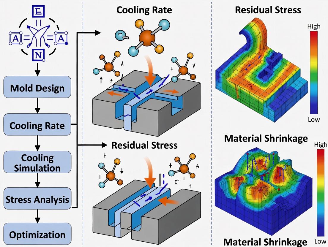
Diagram Title: Cooling Channel Optimization Workflow

Diagram Title: Residual Stress Impact Pathways on Biomedical Parts

The Scientist's Toolkit: Key Research Reagent Solutions & Materials

Item	Function in Residual Stress Research
Photoelastic Coating (Stress Coat)	A brittle coating applied to opaque parts. Cracks under strain provide a qualitative map of surface stress distribution during loading.
Dimethyl Sulfoxide (DMSO) / Ethanol Mixtures	Used as an index-matching fluid in photoelasticity to eliminate surface refraction effects on transparent curved parts.
Strain Gauge Rosette (Type III)	Essential for the hole-drilling method. Precisely measures surface strain relaxation due to material removal.
Low-Modulus, High-Sensitivity Strain Gauges	Required for measuring small strains on compliant polymer materials common in biomedical devices.
Polymer-specific Photoelastic Constant Calibration Kits	Contains known stress specimens to determine the material's stress-optic coefficient (C) for quantitative birefringence.
Annealing Oven with Programmable Profile	For conducting post-molding thermal stress relief studies. Allows systematic study of time-temperature effects on stress relaxation.
Fluorescent Microspheres (for PIV)	Used in mold-filling visualization studies to understand shear history, which contributes to flow-induced residual stress.
Simulated Body Fluid (SBF)	For in vitro aging tests to study the synergistic effect of residual stress and physiological environments on part durability.

Troubleshooting Guides & FAQs

Q1: During my in-mold cooling experiment, I observe inconsistent warpage in my test plaques despite a constant coolant temperature. What is the primary cause and how can I diagnose it?

A: Inconsistent warpage is a direct indicator of non-uniform heat extraction, leading to differential shrinkage and residual stress. The primary cause is likely a maldistribution of coolant flow or varying thermal contact resistance in the cooling channels. To diagnose:

• Map the Temperature Gradient: Use infrared thermography immediately upon part ejection to visualize the surface temperature field. A variation >10°C typically signals problematic non-uniformity.
• Check Flow Rate Balance: Install flow meters on individual cooling circuit branches. Imbalance >15% between parallel channels is a common culprit.
• Inspect for Fouling: Perform a descaling treatment on the cooling channels. Mineral deposits significantly reduce the heat transfer coefficient (HTC).

Q2: My simulation predicts lower residual stress than measured via the layer-removal method. What are the common discrepancies between model and reality?

A: This discrepancy often stems from oversimplified boundary conditions in the simulation.

• Issue: Assumed Perfect Channel Contact. Simulations often use an idealized, constant HTC for all channels. In reality, HTC varies with flow regime (Reynolds Number), channel surface roughness, and possible air gaps.
• Solution: Refine your simulation by implementing a Reynolds-number-dependent HTC correlation (e.g., Dittus-Boelter for turbulent flow) for each channel segment. Correlate your model using a single simple experiment to calibrate the baseline HTC.
• Issue: Neglecting Tool Deformation. The mold itself can warp under non-uniform thermal loads, altering the cavity geometry and cooling gap.
• Solution: Implement a coupled thermal-structural analysis for the mold insert in your simulation to assess this effect.

Q3: How can I experimentally isolate the effect of cooling channel design from material shrinkage properties?

A: Employ a Design of Experiments (DoE) approach using an instrumented mold insert.

• Fixed Material: Use a single, well-characterized material (e.g., a standard polycarbonate) with known PVT (Pressure-Volume-Temperature) data.
• Variable Design: Manufacture multiple inserts with different channel geometries (e.g., straight drilling vs. conformal channels) but identical cavity shapes.
• Direct Measurement: Embed pressure and temperature sensors (e.g., piezoelectric and thermocouple) in the mold wall adjacent to the cavity and near the cooling channels.
• Quantify Stress: For each run, measure residual stress via the layer-removal method on the produced part. The only variable is the cooling channel design, directly linking geometry to stress outcome.

Experimental Protocol: Quantifying Residual Stress via Layer-Removal (Slitting) Method

Objective: To measure the through-thickness residual stress profile in a molded polymer plaque resulting from non-uniform cooling.

Materials & Equipment:

• Injection-molded polymer plaque (e.g., 100mm x 20mm x 4mm).
• Precision strain gauge (uni-axial, Type FLA-2).
• Strain gauge conditioner/amplifier.
• Computerized milling machine or precision wire EDM with depth control.
• Data acquisition system.
• Cyanoacrylate adhesive and strain gauge preparation kit.

Procedure:

• Strain Gauge Bonding: Adhere a strain gauge to the center of the plaque's bottom surface (the surface opposite the initial cut). Ensure perfect alignment along the plaque's long axis.
• Initialization: Connect the gauge to the conditioner and DAQ. Record the stable baseline strain (ε₀).
• Incremental Milling: Secure the plaque in the fixture. Using the milling machine, make a thin, precise cut (slot) on the top surface, increasing the depth in increments (e.g., 0.2mm per step). The cut must be parallel to the strain gauge's transverse axis.
• Strain Recording: After each depth increment, allow thermal equilibration and record the relaxed strain (εᵢ) from the bottom gauge.
• Data Processing: Continue until ~90% of the thickness is cut. Calculate the stress profile using modified integral or differential methods based on measured strain relaxation, elastic modulus (E), and Poisson's ratio (ν) of the material.

Data Analysis Table: Table: Example Strain Data from Layer-Removal Experiment (Polycarbonate, E=2.4 GPa, ν=0.38)

Cut Depth (mm)	Measured Strain (με)	Calculated Stress (MPa)	Notes
0.0 (Baseline)	0	0	Initial state.
0.5	-45	-12.1	Surface in compression.
1.0	-68	-10.8
2.0	-22	5.4	Stress reversal zone.
3.0	+52	14.9	Core in tension.
3.8	+15	4.5	Near final surface.

The Scientist's Toolkit: Research Reagent & Materials

Table: Essential Materials for Cooling Channel & Residual Stress Research

Item	Function & Relevance
Instrumented Mold Insert	A mold tooling insert equipped with embedded thermocouples and pressure transducers to collect real-time in-situ thermal and pressure data during molding.
Phase-Change Thermographic Phosphors	Coatings applied to mold or part surface to measure temperature distributions optically with high spatial resolution, critical for validating thermal simulations.
Low-Pressure Thermoplastic (LPT) Molding Compound	A material with characterized and minimized shrinkage anisotropy, used to isolate cooling effects from material intrinsic shrinkage behavior.
Computational Fluid Dynamics (CFD) Software	To simulate coolant flow, turbulence, and heat transfer coefficients (HTC) within complex cooling channel geometries (e.g., conformal channels).
Structural Stress Mapping Film	A pressure-sensitive film placed in the mold cavity to qualitatively assess uniformity of cavity pressure and, by proxy, packing/cooling effects.

Visualization: Research Workflow for Stress Optimization

Title: Stress Optimization Research Workflow

Title: Stress Buildup from Non-Uniform Cooling

Technical Support Center: Troubleshooting & FAQs

FAQs on Thermal Properties & Processing

Q1: During injection molding of a PLLA stent, we observe premature crystallization leading to brittleness. How can we adjust thermal parameters to control this?

A: Premature crystallization in Poly(L-lactic acid) (PLLA) is often due to improper control of melt and mold temperatures. PLLA has a glass transition temperature (Tg) of ~55-65°C and a crystallization temperature peak (Tc) between 100-120°C.

• Solution: Ensure the melt temperature is maintained above 185°C (but below 240°C to prevent degradation) to erase previous thermal history. The mold temperature is critical: set it between 70-90°C to quench the material into the amorphous state, or precisely between 100-120°C if a specific crystalline content is desired. Use a high cooling rate (>50°C/min) to bypass the crystallization window if an amorphous part is required.

Q2: Our cyclic olefin copolymer (COC) microfluidic devices show flow distortion after autoclaving. What thermal property did we overlook?

A: You have likely approached the Heat Deflection Temperature (HDT) or Vicat Softening Point of the specific COC grade. While COC has a high Tg (up to 180°C), its HDT under load can be significantly lower. Standard autoclaving conditions (121°C, 15-20 psi) can cause deflection if the material is under stress from the mold design.

• Solution: Verify the HDT of your COC grade at the relevant stress (e.g., 0.45 MPa or 1.8 MPa). Select a grade with an HDT at least 15-20°C above the autoclaving temperature. Consider annealing the parts below Tg to relieve molded-in stresses prior to sterilization.

Q3: Differential Scanning Calorimetry (DSC) of a pharmaceutical-grade polymer shows multiple melting endotherms. Is this batch inconsistent?

A: Not necessarily. Multiple endotherms, particularly in polymers like Polyethylene (PE) or Polypropylene (PP), often indicate a distribution of crystalline perfection or different crystal morphologies (e.g., lamellar thickness). This can result from specific catalyst systems or processing conditions.

• Solution: Perform a detailed thermal protocol: First heat (to erase history), controlled cooling, then second heat. If multiple peaks persist on the second heat, it indicates intrinsic polymer structure. Compare the melting enthalpy (ΔHf) between batches quantitatively. Consistency in the total crystallinity (calculated from ΔHf) is more critical than a single peak shape.

Troubleshooting Guide: Experimental Artifacts

Issue: Irreproducible Tg measurements in DSC for a plasticized PVC formulation.

• Potential Cause: Moisture absorption or plasticizer migration. Hydrophilic polymers or those with hygroscopic additives (e.g., PEG) can show depressed and broadened Tg due to water's plasticizing effect.
• Protocol: Follow this standardized drying protocol: Place sample in a vacuum oven at 50°C (below Tg to avoid coalescence) for 24 hours. Store in a desiccator immediately. Load the DSC pan in a dry environment and use a hermetic lid with a pinhole. Run the DSC scan immediately.

Issue: Thermal degradation during melt rheology testing, obscuring viscosity data.

• Potential Cause: Excessive temperature or prolonged exposure in the rheometer barrel, especially for polymers like Polyhydroxyalkanoates (PHA) or Polycaprolactone (PCL).
• Protocol: 1) Conduct TGA first to identify the onset of degradation temperature (Td). 2) Set rheology test temperature at least 30-50°C below Td. 3) Use a nitrogen or argon purge in the rheometer oven. 4) Perform a time-sweep test at the target temperature to establish the safe testing window before viscosity rise.

Data Presentation: Key Thermal Properties of Medical Polymers

Table 1: Thermal Transition Temperatures of Common Medical Polymers

Polymer	Typical Grade	Glass Transition Temp (Tg) °C	Melting Temp (Tm) °C	Degradation Onset (Td) °C	Recommended Processing Window °C
Poly(L-lactic acid)	PLLA	55 - 65	170 - 180	~240	185 - 220
Polycaprolactone	PCL	(-60) - (-65)	58 - 64	~350	80 - 120
Cyclic Olefin Copolymer	COC (Topas 8007)	78	Amorphous	>400	180 - 280
Polyetheretherketone	PEEK 450G	143	343	~580	370 - 400
Medical Polypropylene	Random Copolymer	~0	145 - 155	~300	200 - 240
Ultra-High MW PE	UHMWPE	<-100	130 - 136	~300	200 - 260 (sintering)

Table 2: Thermal Analysis Methods & Standards

Method (ASTM/ISO)	Property Measured	Sample Mass	Heating Rate	Key Output for Medical Polymers
DSC (D3418 / ISO 11357)	Tg, Tm, ΔHf, Crystallinity %	5-10 mg	10°C/min	Degree of crystallinity, sterilization stability
TGA (D3850 / ISO 11358)	Thermal Stability, Filler Content	10-20 mg	10-20°C/min	Residual solvent, decomposition profile
DMTA (D4065 / ISO 6721)	Viscoelastic Moduli vs. Temp	Varies	2-5°C/min	Tan δ peak for Tg, modulus near body temp
HDT (D648 / ISO 75)	Heat Deflection Temp under Load	127 x 13 x 3 mm	120°C/hr	Maximum service temperature for devices

Experimental Protocols

Protocol 1: Determining Crystallinity of a Molded PEEK Component for Surgical Tool

• Objective: Calculate the percentage crystallinity of an injection-molded PEEK part to correlate with its mechanical performance.
• Equipment: Differential Scanning Calorimeter, hermetic aluminum pans, analytical balance.
• Procedure:
  • Precisely weigh 5-8 mg of sample from a specific location on the part (e.g., gate, end-of-fill).
  • Seal sample in a pan. Place in DSC with an empty reference pan.
  • Purge with nitrogen at 50 ml/min.
  • Run temperature cycle: Equilibrate at 30°C. Heat at 10°C/min to 400°C (first heat). Hold for 5 min. Cool at 10°C/min to 30°C. Heat again at 10°C/min to 400°C (second heat).
  • From the second heating curve, identify the melting peak temperature (Tm) and integrate the area to obtain the melting enthalpy (ΔHm, in J/g).
  • Calculate crystallinity: % Crystallinity = (ΔHm / ΔHm°) x 100, where ΔHm° is the melting enthalpy for 100% crystalline PEEK (130 J/g).

Protocol 2: Assessing Polymer Stability for Gamma Sterilization

• Objective: Evaluate the thermal-oxidative stability change in a polypropylene formulation pre- and post-gamma irradiation.
• Equipment: TGA, oxidative atmosphere kit (air or O2), platinum crucibles.
• Procedure:
  • Prepare control and irradiated (typical dose: 25 kGy) samples.
  • Weigh 15-20 mg into a platinum pan.
  • Purge TGA with inert gas (N2) at 60 ml/min. Heat from room temp to 500°C at 20°C/min to record inert degradation profile (optional baseline).
  • Cool back to 100°C.
  • Switch purge gas to dry air or oxygen at 60 ml/min. Hold for 10 min to equilibrate.
  • Heat from 100°C to 600°C at 10°C/min in the oxidative atmosphere.
  • Compare the onset temperature of oxidative degradation (Td_ox) between control and irradiated samples. A decrease of >10°C indicates significant chain scission and increased susceptibility to thermal-oxidative damage.

Mandatory Visualizations

Diagram Title: Thermal Properties Role in Cooling Channel Design Optimization

Diagram Title: DSC Protocol for Crystallinity Measurement

The Scientist's Toolkit: Research Reagent Solutions

Table 3: Essential Materials for Thermal Analysis of Medical Polymers

Item / Reagent	Function / Rationale
Hermetic Aluminum DSC Pans with Lids	To contain the sample and prevent volatile loss (e.g., plasticizer, water) during heating, ensuring data reflects polymer properties only.
Indium Standard (High Purity, 99.999%)	Used for temperature and enthalpy calibration of the DSC. Its sharp melting point (156.6°C) and known ΔHf (28.45 J/g) are reference points.
Nitrogen & Oxidative Gas (Dry Air/O2) Tanks	Inert purge for baseline stability (N2) and oxidative atmosphere for stability testing. Essential for simulating different environments.
Dynamic Mechanical Analysis (DMA) Film Tension Clamp	For measuring viscoelastic properties of thin polymer films or fibers, crucial for understanding performance at body temperature.
Thermal Conductivity Paste	Ensures optimal heat transfer between sensor and sample in Hot Disk or laser flash apparatus for thermal diffusivity measurements.
Microtome or Cryogenic Fracture Tool	To prepare smooth, thin cross-sections of molded parts for localized thermal analysis (e.g., micro-TA, DSC on specific regions like skin vs. core).
Certified Reference Materials (e.g., PE, PP from NIST)	Polymers with certified thermal properties for cross-laboratory validation and instrument performance qualification (PQ).

Technical Support Center: Troubleshooting Guides & FAQs

FAQ 1: Why is my molded polymeric drug delivery device (e.g., microneedle array, implantable reservoir) exhibiting visible surface cracks or hazing after demolding? Answer: This is typically crazing, a precursor to cracking caused by residual tensile stresses exceeding the local yield strength of the polymer. It often occurs due to rapid, non-uniform cooling. In the context of cooling channel optimization, this indicates that the temperature gradient across the part during solidification is too steep. Crazing can create micro-pathways, leading to uncontrolled drug elution rates and potential sterility breaches.

FAQ 2: Our molded parts fail to meet dimensional specifications, showing warpage that affects assembly. How is this linked to our injection molding process? Answer: Warpage is a direct consequence of differential residual stress (often shrinkage) through the part thickness. This is fundamentally controlled by the cooling phase. Sub-optimal cooling channel design leads to asymmetric cooling rates between the core and cavity sides of the mold. The side that cools and solidifies first constrains the later-cooling side, inducing bending moments. This compromises the fit and function of assembled drug delivery systems.

FAQ 3: During in vitro testing, our device fractures under simulated physiological loads. What failure mode is this, and how can molding stresses contribute? Answer: This is a brittle fracture failure mode. High residual stresses, particularly frozen-in tensile stresses from packing and cooling, act as a pre-load on the material. This reduces the effective stress required from external loads to reach the material's fracture toughness. Optimized cooling reduces these baseline stresses, thereby increasing the device's functional safety factor.

FAQ 4: We observe batch-to-batch variability in drug release profiles. Could molding artifacts be a root cause? Answer: Absolutely. Stress-induced warpage can alter fluid flow paths within microfluidic channels. More subtly, crazing creates a network of micro-cracks that can significantly increase the surface area for drug diffusion or create unintended capillary action, accelerating release. Consistent, stress-minimized molding is critical for reproducible release kinetics.

Experimental Protocols for Stress Analysis

Protocol 1: Photoelasticity for Qualitative Stress Visualization

• Material: Fabricate test parts from a transparent, birefringent polymer (e.g., polycarbonate, epoxy).
• Setup: Place the part between two polarizing filters in a polariscope.
• Procedure: Subject the part to simulated service loads (or analyze as-molded). Observe the fringe patterns (isochromatics) that develop.
• Analysis: The number and density of fringes are proportional to the magnitude of shear stress. Concentrated fringe patterns indicate high-stress zones likely to initiate failure.
• Link to Cooling: Compare fringe patterns from parts molded with different cooling channel layouts (e.g., straight-drilled vs. conformal channels).

Protocol 2: Warpage Measurement using Coordinate Measuring Machine (CMM)

• Equipment: A precision CMM with a non-contact (laser) or touch-trigger probe.
• Baseline: Program the CMM with the CAD nominal dimensions of the part.
• Measurement: Secure the molded part on the CMM table. Probe critical points on the surface (e.g., corners, midpoints of edges).
• Data Processing: Software calculates the deviation of each point from its nominal position.
• Quantification: The maximum deflection (flatness error) and the pattern of deviation are quantified. Data is used to validate computational models of cooling.

Protocol 3: Accelerated Drug Release Testing for Crazing Impact

• Sample Preparation: Produce two sets of devices: one molded under standard cooling (prone to crazing) and one under optimized, stress-reducing cooling.
• Load: Load each device with a standard amount of model drug (e.g., fluorescein).
• Release Medium: Immerse devices in a standard buffer (e.g., PBS pH 7.4) at 37°C under gentle agitation.
• Sampling: Withdraw aliquots at predetermined time intervals (e.g., 1, 3, 6, 12, 24 hrs).
• Analysis: Quantify drug concentration via UV-Vis spectroscopy or HPLC.
• Comparison: Compare release profiles. A significantly faster release in the standard-cooled batch indicates craze-induced diffusion pathways.

Data Presentation

Table 1: Impact of Cooling Channel Design on Measured Part Quality Attributes

Cooling Channel Type	Average Warpage (µm)	Crazing Incidence (% of batches)	Burst Pressure Failure (avg. MPa)	Drug Release Rate (k, hr⁻¹)
Standard Straight Drilled	245 ± 35	45%	2.1 ± 0.3	0.52 ± 0.07
Spiral Conformal	115 ± 22	10%	3.0 ± 0.2	0.31 ± 0.04
Hybrid (Baffle+Serial)	85 ± 18	5%	3.4 ± 0.3	0.28 ± 0.02

Data is representative of PLA-based implantable reservoirs molded at 65°C mold temperature. Drug release modeled as first-order kinetics.

Table 2: The Scientist's Toolkit: Key Reagents & Materials for Stress-Resilient Device Development

Item	Function in Research
Birefringent Polymer (e.g., Polycarbonate)	Allows for direct visualization of residual stresses via photoelasticity.
Poly(L-lactide) (PLLA) / PLGA Resins	Model biodegradable polymers for implantable drug delivery devices.
Fluorescein Sodium Salt	A hydrophilic model drug compound for tracking release kinetics.
PBS Buffer Tablets (pH 7.4)	Provides a physiologically relevant medium for in vitro release testing.
Digital Shim Stock (Various Thicknesses)	Used to create intentional, variable wall thicknesses in mold designs to study cooling effects.
Mold Temperature Controller	Precisely controls coolant temperature, a critical variable in residual stress formation.
Finite Element Analysis (FEA) Software (e.g., ANSYS, Moldex3D)	Simulates cooling, predicts warpage, and optimizes channel design before tooling fabrication.

Visualizations

Title: Stress Pathway from Cooling to Device Failure

Title: Workflow for Cooling Channel Optimization Research

From Simulation to Reality: Methodologies for Designing Stress-Minimizing Cooling Systems

Within the thesis research on Optimizing cooling channel design for residual stress reduction in molded parts, Computer-Aided Engineering (CAE) tools are indispensable. This technical support center provides targeted troubleshooting and FAQs for researchers and scientists using Autodesk Moldflow and Moldex3D to simulate residual stresses, a critical factor affecting part warpage, dimensional stability, and mechanical integrity.

Troubleshooting Guides & FAQs

Q1: Why does my residual stress simulation show unrealistic, highly localized stress concentrations near the gates?

A: This is often due to excessive mesh refinement in gate regions combined with default solver settings. The high shear heating and rapid freezing are not properly captured.

• Solution:
  • Mesh Check: Ensure the mesh transition from the gate to the part body is gradual. Avoid extreme element size ratios (>5:1).
  • Process Settings: Verify that the injection time and velocity profile are physically realistic. An overly fast fill can exaggerate shear stresses.
  • Material Data: Confirm the viscosity and PVT data for your polymer is accurate and covers the relevant shear rate and temperature ranges.
  • Solver Adjustment: In Moldex3D, enable the "Enhanced Warpage" calculation. In Moldflow, ensure "Residual Stress" analysis is selected in the warpage sequence.

Q2: How do I validate simulated residual stress results against experimental data (e.g., layer removal, photoelasticity)?

A: Direct comparison requires mapping simulation data to the experimental method.

• Protocol for Layer Removal Validation:
  • Simulation: Run a full Cool + Fill + Pack + Warp analysis. Export the in-mold stress tensor (stress at ejection) for the part cross-section.
  • Experiment: Machine thin layers from the part surface and measure the curvature after each removal step.
  • Correlation: Use the classical integral equation from the layer removal theory. Input your simulated through-thickness stress profile to calculate the predicted curvature change. Compare this curve to your experimental curvature measurements.

Q3: My cooling channel design optimization is not reducing residual stress as expected. What parameters are most sensitive?

A: Cooling uniformity is more critical than absolute temperature. Focus on temperature differentials across the part.

• Solution Workflow:
  • Run a baseline cooling analysis.
  • Extract the part temperature distribution at ejection.
  • Identify high-gradient zones. These are primary residual stress drivers.
  • Optimize by adjusting channel pitch, depth from surface, and circuiting to minimize the temperature difference (ΔT). A table of iterative results is crucial.

Q4: What is the difference between "Flow-induced" and "Thermally-induced" residual stress in CAE results, and how are they computed?

A: CAE tools decompose the total stress.

• Flow-induced (Shear) Stress: Generated during the filling/packing phases due to viscoelastic polymer flow under shear and elongation. Calculated from the flow kinematics and constitutive model.
• Thermally-induced (Thermal) Stress: Dominant contributor, arising from differential cooling and shrinkage constraints. Calculated based on the temperature history, PVT behavior, and modulus development.
• Key: The solver integrates these effects through a thermo-viscoelastic stress model during the cooling phase. Ensure your material model supports this (e.g., modified Cross-WLF with stress relaxation).

Experimental Protocol: Correlating Cooling Design to Residual Stress

Objective: Quantify the impact of cooling channel layout on residual stress magnitude and distribution for a test plaque.

Methodology:

• CAE Simulation Phase:
  • Model: Create a 150mm x 100mm x 3mm plaque model with a single edge gate.
  • Design of Experiments (DOE): Define three cooling channel configurations:
    • Design A: Standard parallel channels.
    • Design B: Conformal channels closer to the part surface.
    • Design C: Baffled channels for high-heat areas.
  • Analysis Sequence: Run identical Fill + Pack + Cool + Warp analyses for each design in both Moldflow and Moldex3D.
  • Output: Extract the volumetric shrinkage and principal stress (σ1) at ejection. Calculate the average and range of stress across the part mid-plane.

• Data Synthesis: Compare results using the table below.

Table 1: Cooling Design Impact on Simulated Residual Stress

Cooling Design	Channel Depth (mm)	Part ΔT at Ejection (°C)	Max Principal Stress (MPa)	Stress Uniformity (Std. Dev.)	Predicted Warpage (mm)
A: Parallel	15	42.5	28.7	8.2	1.45
B: Conformal	10	24.1	19.3	4.1	0.82
C: Baffled	12	28.7	21.5	5.3	0.97

Visualizing the Residual Stress Simulation Workflow

Diagram Title: CAE Workflow for Residual Stress in Molding

The Scientist's Toolkit: Research Reagent Solutions

Table 2: Essential Materials & Software for Residual Stress Research

Item/Category	Function & Relevance to Research
High-Performance Polymer (e.g., Polycarbonate, PMMA)	Amorphous polymers show pronounced residual stresses and are ideal for method development and photoelastic validation.
Photoelasticity Setup (Polarizer, Light Source, Birefringent Material)	Provides full-field visual validation of residual stress patterns (isochromatic fringes) in transparent models or parts.
Strain Gauges & Data Logger	For quantitative validation of warpage and strain recovery in layer-removal or hole-drilling experiments.
Autodesk Moldflow Insight	Industry-standard CAE for simulating the molding process. Its "Residual Stress" module is key for this thesis.
Moldex3D Studio	Advanced CAE with robust 3D solvers for accurate prediction of cooling-induced stresses and deformations.
MATLAB or Python (with NumPy/SciPy)	For post-processing simulation data, performing statistical analysis on DOE results, and implementing custom stress analysis algorithms.
Digital Scanning (CT or Laser)	To obtain precise as-built geometry for comparison with simulated warpage, closing the validation loop.

Technical Support Center: Troubleshooting & FAQs

This support center addresses common experimental challenges encountered when designing and implementing conformal cooling channels (CCCs) for research on residual stress reduction in molded parts. The guidance is framed within a thesis context focusing on optimizing cooling channel design.

Frequently Asked Questions (FAQs)

Q1: During thermal simulation of our CCC design, we observe unexpected "hot spots" near sharp internal corners. What is the likely cause and how can we resolve it? A: This is a common issue related to fluid dynamics and heat transfer principles. The cause is a decrease in local coolant velocity and potential flow separation in sharp bends, reducing heat extraction efficiency.

• Solution: Redesign the channel path to maintain a consistent cross-sectional area and implement a minimum bend radius of 1.5 times the channel diameter. For corners, use gradual arcs instead of sharp angles. Verify the improvement using Computational Fluid Dynamics (CFD) simulation before manufacturing.

Q2: Our metal 3D-printed CCC insert shows premature failure or cracking during cyclic injection molding trials. What should we investigate? A: This typically points to issues with the additive manufacturing (AM) process parameters or post-processing.

• Troubleshooting Checklist:
  • Material & Stress: Verify the stainless steel (e.g., 1.2709) or tool steel powder is within specification.
  • Print Parameters: Review laser power and scanning strategy with your AM provider; sub-optimal settings can create internal defects.
  • Residual Stress from AM: Ensure the insert underwent stress relief annealing immediately after printing.
  • Surface Roughness: Internally rough channels act as stress concentrators. Specify and measure internal surface roughness (Ra), aiming for Ra < 10 µm via abrasive flow finishing if necessary.
  • Support Structure Removal: Inspect for tool marks or cracks originating from support removal points inside channels.

Q3: How do we accurately measure the residual stress in our molded test plaques to quantify the benefit of our CCC design? A: This requires a controlled experimental protocol.

• Recommended Protocol: Semi-Destructive Hole-Drilling Strain Gauge Method.
  • Sample: Mold identical plaques using both the CCC insert and a conventional straight-drilled channel insert under identical process parameters (melt temp, pack pressure, cycle time).
  • Preparation: Attach a specialized three-element strain gauge rosette to the plaque surface at critical points (e.g., near gates, thick sections).
  • Drilling: Use a high-speed air turbine drill with a 2mm diameter end mill to incrementally drill a shallow hole in the center of the rosette. This relieves residual stresses.
  • Measurement: A strain gauge data logger records the released strains at each drilling increment.
  • Analysis: Apply ASTM E837 standard calculations to convert measured strains into residual stress magnitude and direction. Compare results between CCC and conventional cooling samples.

Q4: We are encountering clogging in our CCCs during long-term molding experiments. How can we prevent this? A: Clogging is often due to mineral scale or corrosion byproducts.

• Preventive Actions:
  • Coolant Treatment: Use deionized water with anti-corrosion and anti-scaling additives. Maintain pH between 7.5 and 8.5.
  • Filtration: Install a 5-10 micron inline filter in the coolant loop.
  • Channel Design: Avoid internal support structures that are not fully removed and design channels with self-cleaning, smooth paths.
  • Startup Procedure: Always flush the cooling system thoroughly before connecting to a new CCC insert.

Data Presentation: Key Performance Metrics

Table 1: Quantitative Comparison of Cooling Channel Performance in a Representative Study

Metric	Conventional Drilled Channels	Conformal Cooling Channels (CCCs)	Measurement Method
Cooling Time Reduction	Baseline (0%)	20% - 40%	In-mold thermocouple, cycle timing
Part Warpage Reduction	Baseline	30% - 60%	Coordinate Measuring Machine (CMM)
Maximum Residual Stress	High (Reference)	25% - 50% lower	Hole-drilling strain gauge (ASTM E837)
Surface Temperature Variation	High (± 15°C)	Low (± 3°C)	Thermal imaging camera during cycle
Typical Achievable Ra (Roughness)	< 1.25 µm (machined)	6 - 15 µm (as-printed)	Profilometer on sectioned channel

Experimental Protocol: Validating CCC Performance

Title: Protocol for Comparative Thermal Cycling and Warpage Analysis

Objective: To quantitatively assess the cooling efficiency and part quality improvement of a CCC insert versus a baseline insert.

Materials:

• Two identical mold cores: one with CCCs (Test), one with straight drilled channels (Control).
• Injection molding machine.
• In-mold temperature sensors (4 per insert, placed at critical locations).
• Thermal imaging camera.
• Polypropylene or ABS resin (consistent lot).
• Coordinate Measuring Machine (CMM).

Method:

• Instrumentation: Install both inserts sequentially. Embed temperature sensors at identical geometric locations relative to the cavity.
• Process Stabilization: For each insert, establish a stable molding process at recommended parameters. Record melt temperature, injection speed, packing pressure, and cooling time.
• Data Collection Cycle:
  • Mold 50 consecutive parts to achieve thermal equilibrium.
  • For parts 51-100, record: (a) Temperature curves from all sensors, (b) A thermal image of the part surface upon ejection using the thermal camera.
  • Measure parts 91-100 using CMM after 24 hours of conditioning to assess warpage (flatness deviation).
• Analysis: Calculate average cooling time to ejection temperature. Compare temperature uniformity (standard deviation across sensors). Analyze warpage data statistically (e.g., t-test on CMM deviation data).

Visualization: Research Workflow

Diagram Title: CCC Research Workflow for Residual Stress Reduction

The Scientist's Toolkit: Key Research Reagent Solutions

Table 2: Essential Materials & Equipment for CCC Research

Item	Function in Research	Specification Notes
Metal Powder (for AM)	Raw material for printing CCC inserts.	Maraging Steel (1.2709) is common; offers high strength and good thermal conductivity post-ageing.
Abrasive Flow Finishing Media	Polishes internal channel surfaces to reduce roughness and improve flow.	Silicon carbide or boron carbide-based medium. Viscosity selected based on channel diameter.
Coolant Additive Kit	Prevents corrosion and scaling within CCCs during long-term trials.	Must be compatible with deionized water and the printed metal alloy (e.g., nitrite-free for stainless steel).
Strain Gauge Rosette (Type TE)	Measures strain relieved during hole-drilling for residual stress calculation.	Follow ASTM E837; Type TE rosettes with a 1/16" gauge length are typical for plastics.
High-Temperature Epoxy	Bonds strain gauges to molded plastic parts for stress measurement.	Must have a thermal expansion coefficient similar to the polymer under test to avoid artifact strains.
In-Mold Temperature Sensor	Directly measures coolant and mold temperature at critical points.	Use fast-response, sheathed thermocouples (J or K type) capable of >150°C.

Technical Support Center

Troubleshooting Guides

Issue: Inconsistent Part Temperature After Molding

• Problem: Residual stress analysis shows high, uneven distribution in complex geometric regions (e.g., ribs, bosses) despite using baffles.
• Potential Causes & Solutions:
  • Baffle Channel Blockage: Debris or mineral scale is obstructing the internal fins of the baffle. Action: Perform a citric acid (5-10%) flush of the cooling circuit and install a 50-micron inline filter.
  • Insufficient Flow Rate: The pressure drop across the baffle is too high, reducing coolant velocity and heat transfer. Action: Refer to Table 1. Increase pump pressure or consider a parallel circuit layout for high-drop components.
  • Air Lock (Bubble Formation): Vapor traps in the baffle's upstream leg prevent coolant contact. Action: Ensure the baffle is oriented vertically, with outlet at the top to vent air. Install automatic air vents at circuit high points.

Issue: Thermal Pin (Heat Pipe) Performance Degradation

• Problem: Measured thermal conductivity of the thermal pin drops below manufacturer specification (>5,000 W/m·K), leading to hot spots.
• Potential Causes & Solutions:
  • Non-Condensable Gas (NCG): Degradation of the internal working fluid generates gases that impede the condensation cycle. Action: Replace the thermal pin. Monitor mold temperature to avoid sustained operation above the pin's maximum rated temperature.
  • Improper Interface Contact: Poor fit between the pin's condenser end and the cooling channel reduces heat sink efficiency. Action: Apply a high-thermal-conductivity interface paste (see Scientist's Toolkit) and ensure machining tolerances are within ±0.05mm for press-fit installations.

Issue: Oscillating Temperature Readings with Bubble-Driven Flow

• Problem: When using a bubble-driven agitation system (e.g., for a conformal channel), temperature sensors show cyclical variations >±2°C.
• Potential Causes & Solutions:
  • Unstable Bubble Generation: Inconsistent gas injection rate or bubble size. Action: Calibrate the piezoelectric injector or sintered metal sparger. Use a high-speed camera to verify bubble generation uniformity against protocol.
  • Resonant Frequency Interference: The bubble release frequency matches the natural frequency of the sensor mount. Action: Adjust the gas pulse frequency by 10-15% and dampen the sensor mounting point.

Frequently Asked Questions (FAQs)

Q1: What is the optimal placement ratio for baffles in a deep-core region to minimize residual stress? A: Based on recent studies (see Table 1), for core geometries with an aspect ratio (depth/diameter) >4, a staggered placement of baffles at a pitch-to-diameter ratio of 2.5-3.0 provides the most uniform cooling. This typically reduces in-plane residual stress variance by 15-20% compared to a single central baffle.

Q2: How do I calculate the required pressure for a bubble-agitated conformal channel? A: The driving pressure (ΔP) must overcome surface tension and hydrostatic pressure. Use the modified Young-Laplace equation: ΔP = (2σ/r) + ρgh + ΔPfriction, where σ is surface tension, r is the bubble radius, ρ is coolant density, g is gravity, h is channel depth, and ΔPfriction is the laminar flow pressure drop. A safety factor of 1.3 is recommended.

Q3: Can thermal pins be used in a pulsed cooling regime for stress management? A: Yes, but their response is limited by the sonic velocity of the internal vapor. Typical activation time is 0.5-2 seconds. For pulses faster than 1 Hz, the effective conductivity drops, and a steady-state thermal simulation should be used. See the experimental protocol below for testing transient response.

Q4: What is the most common failure mode for polymer-based cooling channel inserts in drug device molding? A: Delamination or creep at the metal-polymer interface due to cyclic thermal stress. Regular inspection with a borescope is advised. Failure typically manifests as a >10% gradual increase in part temperature at the same inlet coolant temperature.

Data Presentation

Table 1: Performance Comparison of Advanced Cooling Components

Component	Typical Thermal Conductivity / Efficacy	Optimal ΔP Range	Max Aspect Ratio	Avg. Residual Stress Reduction*
Standard Drilled Channel	-	0.5 - 1.5 bar	~1:1	Baseline (0%)
Baffle (Internal Finned)	Effective Conductivity: 3-5x of channel	1.8 - 3.0 bar	Up to 8:1	25-30%
Bubble-Agitated Channel	Heat Transfer Coeff. Increase: 40-70%	0.2 - 0.7 bar (gas)	Conformal	15-20%
Thermal Pin (Copper/Water)	Effective Conductivity: >5,000 W/m·K	N/A (Passive)	Up to 20:1	30-40% (in localized hotspots)

*Measured via hole-drilling method on polycarbonate test plaques with a rib feature.

Experimental Protocols

Protocol 1: Evaluating Baffle-Induced Cooling Uniformity Objective: Quantify the effect of baffle pitch on part temperature gradient and residual stress.

• Tooling: Fabricate a mold with a 100mm deep, 20mm diameter core pin. Install three vertically placed, interchangeable baffles with pitch-to-diameter ratios of 2.0, 2.5, and 3.0.
• Instrumentation: Embed five K-type thermocouples along the core sidewall at 20mm intervals. Connect to a data logger.
• Process: Inject Polypropylene (PP) at 230°C. Maintain coolant (water) at 25°C and a constant flow rate of 4 L/min.
• Data Collection: Record the temperature profile during cooling until ejection (80°C). Produce 10 parts per configuration.
• Stress Analysis: Use a hole-drilling strain gauge apparatus (ASTM E837) on the ejected part's corresponding surface. Calculate the principal stress magnitude and gradient.

Protocol 2: Characterizing Thermal Pin Transient Response Objective: Measure the effective thermal conductivity of a thermal pin under pulsed heating.

• Setup: Mount a 6mm diameter, copper/water thermal pin in an insulating (ceramic) block. Apply a calibrated cartridge heater (500W) to the evaporator end. Attach a water-jacketed cold plate to the condenser end (15°C).
• Pulsing: Use a programmable DC power supply to apply a square wave heating pulse: 300W for 5s, 0W for 10s. Repeat for 10 cycles.
• Measurement: Record temperatures at the evaporator (Tevap) and condenser (Tcond) junctions at 100Hz.
• Calculation: During the on pulse, calculate effective conductivity: keff = (Q * L) / (A * (Tevap - Tcond)), where Q is heat input, L is pin length, A is cross-sectional area. Plot keff over time to observe stabilization.

Mandatory Visualization

Diagram Title: Cooling Component Selection Workflow for Stress Reduction

Diagram Title: Bubble-Driven Cooling Enhancement Pathway

The Scientist's Toolkit: Research Reagent Solutions

Item	Function in Cooling Circuit Research
Degassed, Deionized Water	Primary coolant fluid; degassing prevents bubble nucleation that interferes with flow and heat transfer measurements.
Thermal Interface Paste (e.g., Zinc Oxide Silicone Grease)	Ensures minimal thermal contact resistance between thermal pins/inserts and the mold base.
Citric Acid Solution (5-10% w/v)	Safe, biodegradable agent for descaling and removing mineral deposits from cooling channels without corrosion.
Non-Reactive Tracer Dyes (Rhodamine WT, Fluorescein)	Used in flow visualization experiments to map coolant flow paths and identify stagnation zones in complex circuits.
Polyvinyl Alcohol (PVA) Soluble Inserts	Used to create conformal cooling channels in trial molds; dissolved post-fabrication to leave complex internal passages.
Strain Gauge Rosettes (Type EA-XX-xxx)	Applied directly to molded parts for residual stress measurement via the hole-drilling strain relaxation method (ASTM E837).

Technical Support Center

Troubleshooting Guides & FAQs

Q1: During injection molding of a microfluidic chip, we observe high residual stresses leading to warpage. The part fails to seal properly in the bonding step. What is the primary cooling-related factor? A: Non-uniform cooling is the most likely cause. If the cooling rate differs significantly across the part, thermal gradients induce uneven shrinkage, locking in tensile and compressive stresses. This is exacerbated in molds with complex, thin-walled geometries like microfluidic channels. Ensure your cooling channels follow the part contour as closely as possible (conformal cooling) and check for balanced flow rates in all channel circuits.

Q2: Our inhaler actuator mold produces parts with visible sink marks near thick sections. Adjusting pack pressure and time hasn't resolved it. How can cooling optimization help? A: Sink marks occur when the inner material cools and shrinks after the outer skin has solidified. Inadequate cooling in thick sections prolongs this phase. Optimizing cooling involves increasing the cooling time specifically for these regions, often by placing baffles or bubblers to direct coolant flow directly into cores opposing the thick sections. The goal is to reduce the temperature difference between the thick and thin sections at ejection.

Q3: We are designing a new mold for a PLGA microfluidic device. What quantitative metrics should we use to evaluate cooling channel design performance? A: Key metrics for evaluation include:

Metric	Target for Microfluidic/Inhaler Molds	Measurement/Simulation Method
Cooling Time	Minimize, but maintain uniformity	Moldflow analysis, analytical calculation
Part Temperature Variance at Ejection	< 10°C across the part	Transient thermal simulation (e.g., ANSYS, Moldex3D)
Coolant Temperature Rise	< 5°C between inlet and outlet	Experimental measurement, CFD
Maximum Residual Stress	Minimize, target < 50% of material yield strength	Structural FEA with thermal loads (e.g., Abaqus)
Cooling System Pressure Drop	< 2 bar for standard systems	CFD, empirical equations

Q4: What is a step-by-step protocol for experimentally validating cooling efficiency and its effect on residual stress in a newly fabricated mold? A: Protocol: Thermal Imaging and Warpage Analysis for Mold Validation

• Instrumentation: Install the mold in an injection molding machine fitted with pressure/temperature sensors in the coolant lines. Prepare a thermal imaging camera (FLIR).
• Baseline Run: Run a short shot (95% fill) at standard process settings. Eject the part and immediately capture a full-field thermal image. Record coolant inlet/outlet temperatures and pressures.
• Warpage Measurement: Using a coordinate measuring machine (CMM) or laser scanner, measure the geometry of a fully cooled part against the CAD model. Map deviation.
• Stress Analysis via Layer Removal: For a flat section (e.g., an inhaler baseplate), mill away thin, parallel layers from one side. Measure the curvature change after each removal. Use beam bending theory to back-calculate the through-thickness residual stress profile.
• Correlation: Correlate areas of high residual stress with areas of high initial temperature or high cooling gradient from the thermal images.
• Iterate: Adjust coolant flow rates or temperatures to improve uniformity and repeat the cycle.

Q5: Are conformal cooling channels always the best solution for reducing residual stress in microfluidic molds? A: Not always. While conformal channels provide excellent thermal uniformity for complex geometries, their manufacturing (via additive manufacturing like DMLS) can introduce surface roughness, leading to poor heat transfer if not polished. They can also be prone to clogging if coolant water quality is poor. For simpler planar microfluidic designs, a well-designed traditional drilled channel system with thermal inserts may be equally effective and more robust. A cost-benefit analysis considering part quality, mold lifespan, and manufacturing cost is essential.

Research Reagent & Essential Materials Toolkit

Item	Function in Cooling Optimization Research
Simulation Software (ANSYS, Moldex3D)	For virtual DOE of cooling channel layouts, predicting temperature fields, cooling times, and warpage.
Additively Manufactured Mold Inserts (e.g., Maraging Steel 1.2709)	Enable fabrication of complex conformal cooling channels unachievable with drilling.
Thermochromic Liquid Crystal (TLC) Films or Paints	Applied to the mold or part surface to visually map temperature distributions in real-time during molding.
Strain Gauge Rosettes & Data Logger	Bonded to the mold or part (if accessible) to measure strain during cooling, used to calculate stress.
Polycarbonate (PC) or PMMA Resin	Common, transparent model materials for prototyping molds and visualizing flow and cooling effects.
High-Thermal-Conductivity Mold Materials (e.g., Copper Alloys, Aluminium 7075)	Used for critical inserts to enhance heat extraction in localized hot spots.
Non-Newtonian Coolant Additives	To improve heat transfer coefficients in turbulent flow regimes within narrow cooling channels.
Polariscope (Photoelasticity Setup)	For qualitative full-field visualization of residual stresses in transparent prototype parts (e.g., PMMA).

Experimental & Analysis Workflows

Title: Cooling Channel Design Optimization Workflow for Stress Reduction

Title: Causal Pathway from Poor Cooling to Part Failure

Solving Cooling Imbalances: A Troubleshooting Guide for Stress Reduction

Troubleshooting Guides & FAQs

Q1: During injection molding of a complex microfluidic device prototype, we observe warpage and dimensional inaccuracy in specific channels. How do we determine if this is due to a localized hot spot or differential cooling?

A: This is a classic symptom of thermal imbalance. Follow this diagnostic protocol:

• Instrument the Mold: Embed micro-thermocouples (Type K, 80μm sheathed) at suspected locations (gate, end-of-fill, thick sections) and in a known stable area for reference.
• Map Temperature Delta: Conduct 10 consecutive molding cycles. Record the peak temperature and the time to cool to ejection temperature (e.g., 80°C) for each sensor.
• Analyze: A persistent temperature delta >15°C between a sensor and the reference at the time of ejection indicates a hot spot. Correlate these sensor locations with the warped features on the part.

Q2: Our molded polymer test coupons show sink marks and internal voids. Does this point to a cooling channel design flaw or an injection parameter issue?

A: Sink marks and voids often result from differential shrinkage where internal material cools and shrinks faster than the surface. To isolate the cause:

• First, optimize packing pressure and time in a Design of Experiment (DoE) approach to ensure adequate material compensation.
• If defects persist, the issue is likely cooling. Perform a short-shot experiment (90% fill). If the unfilled section corresponds to the defect area, the local cooling rate is excessive, causing premature solidification and preventing pack-out.
• Validated Solution: Redesign cooling channels to maintain a more uniform mold surface temperature, typically within ±5°C of the target.

Q3: What is the most reliable experimental method to quantify residual stress induced by thermal gradients in a transparent part?

A: The industry standard is Photoelasticity.

• Protocol: Use an optically clear material (e.g., PMMA). Place the molded part between crossed polarizers in a polariscope.
• Procedure: Apply a calibrated tensile load to the part until the fringe pattern matches its as-molded state. The magnitude of the applied stress required is equivalent to the residual stress locked in the part. Record fringe order and pattern location.
• Quantification: Use the stress-optic law: σ = N * f / t, where N is fringe order, f is material fringe value (e.g., 7.2 kN/fringe for PMMA), and t is thickness.

Data Presentation

Table 1: Impact of Cooling Channel Design on Key Quality Metrics

Cooling Design	Distance from Cavity (mm)	ΔT Mold Surface (°C)	Part Warpage (mm)	Max Residual Stress (MPa)
Straight Drilled	15	±12.5	0.87	24.5
Conformal (3D Printed)	8	±4.2	0.21	8.7
Baffle-Cascade	12	±7.8	0.49	15.3

Table 2: Defect Root Cause & Diagnostic Signature

Observed Defect	Probable Thermal Cause	Diagnostic Tool	Key Metric
Warpage/Bending	Non-uniform cooling, hot spot on one side	Mold Temp Sensors, Thermal Imaging	Temp Delta >15°C across part
Sink Marks	Local over-cooling, premature gate freeze	Short-shot Study, Pressure Trace	Pack time < local solidification time
Voids	High core temp, low surface temp (differential shrinkage)	CT Scan, Sectioning	Density variation >5% in core vs. skin
Weld Lines	Low melt temp at flow front due to heat loss	High-Speed IR Camera	Melt front temp drop >30°C

Experimental Protocols

Protocol: Thermal Imaging for Hot Spot Identification

• Objective: Visually map the mold surface temperature distribution during cycling.
• Materials: Mid-wave IR camera (3–5 μm spectral range), emissivity calibration tape (ε=0.95), injection molding machine.
• Method: a. Apply calibration tape to several locations on the mold surface. b. Set camera to correct for material emissivity (steel ≈0.15-0.25, use tape for calibration). c. Record thermal video starting from mold open, through close, injection, cooling, and open. d. Analyze frame-by-frame to identify areas that remain >10% hotter than the average mold temperature during the cooling phase.
• Output: False-color thermal map with isotherms highlighting hot spots.

Protocol: Measuring Differential Shrinkage via Coordinate Measuring Machine (CMM)

• Objective: Quantify dimensional variation due to non-uniform cooling.
• Materials: CMM (5μm accuracy), thermally stabilized part (24 hrs at 23°C/50% RH), CAD nominal model.
• Method: a. Measure critical dimensions (e.g., channel width, wall thickness) at 10 predefined locations. b. Compare to nominal dimensions from CAD. c. Calculate linear shrinkage: S = (Dmold - Dpart) / D_mold * 100%. d. Plot shrinkage values against their relative distance from the cooling channels.
• Output: Shrinkage distribution map correlating high-variation zones with distant or inefficient cooling.

Mandatory Visualization

Diagram: Thermal Imbalance Defect Diagnosis Workflow

Diagram: Key Factors in Cooling Channel Optimization

The Scientist's Toolkit: Research Reagent Solutions

Table 3: Essential Materials for Thermal Imbalance Research

Item	Function & Specification
Micro-thermocouples (Type K)	For direct, real-time temperature measurement within the mold or part. Sheathed (80-150μm) for minimal intrusion.
High-Speed Infrared Camera	For non-contact, full-field thermal mapping of mold or part surface. Requires MWIR (3-5μm) range for metals.
Photoelastic Polariscope	For visualizing and quantifying residual stress fields in transparent polymers via birefringence.
Coordinate Measuring Machine (CMM)	For high-precision (μm-level) measurement of part geometry and calculation of local shrinkage.
Conformal Cooling Mold Insert	3D-printed (e.g., SLM from tool steel) insert with channels following the part contour for uniform cooling.
Thermally Stable Masterbatch	Additives (e.g., fluorescent dyes) for flow front tracking, or calibrated shrinkage modifiers for study.
Mold Filling & Cooling Simulation Software	Finite Element Analysis (FEA) tool to predict melt flow, cooling time, and warpage before physical trials.

Technical Support Center: Troubleshooting & FAQs

This support center provides guidance for issues related to the optimization of cooling channel parameters in injection molding, specifically within a research context focused on minimizing residual stress in molded parts for advanced applications, including medical and pharmaceutical device components.

Frequently Asked Questions (FAQs)

Q1: During our thermal cycling experiments, we observe inconsistent cooling and warpage in the molded part. We suspect the coolant flow rate is insufficient. What is the recommended starting point for flow rate to achieve turbulent flow in micro-scale channels? A: For water-based coolants, aim for a Reynolds Number (Re) > 4000 to ensure turbulent flow, which maximizes heat transfer. As a rule of thumb, for a channel diameter of 10 mm, a flow velocity of > 0.4 m/s is typically required. Use the formula Re = (ρ * v * D) / μ, where ρ is density, v is velocity, D is diameter, and μ is dynamic viscosity. Start with a flow rate (Q) calculated from your target velocity and channel cross-sectional area (Q = v * A). Monitor pressure drop to ensure it remains within your system's limits.

Q2: Our simulation results show high residual stress near the channel walls, contradicting our goal. Could the channel pitch be the issue? A: Yes, an excessively large pitch creates significant temperature gradients between channels, leading to uneven cooling and high thermal stresses. A pitch that is too small can cause overcooling and high interfacial shear stress. As a baseline, the pitch-to-diameter ratio (P/D) should be between 2 and 3 for uniform cooling. Refer to the quantitative data table for specific findings.

Q3: What is the optimal channel depth from the mold cavity surface to balance cooling efficiency and mold strength? A: The depth ratio (distance from cavity surface to channel center, divided by channel diameter) is critical. A ratio between 0.75 and 1.5 is generally optimal. A depth too shallow (<0.5D) risks surface deflection and non-uniform cooling, while a depth too deep (>2D) reduces cooling efficiency. For a 8 mm diameter channel, a depth of 6-12 mm from the surface is a common effective range.

Q4: How do we validate that our optimized parameters are effectively reducing residual stress in the final part? A: Implement a combined experimental protocol: First, use moldflow analysis to simulate residual stress based on your parameters. Second, manufacture a mold with your optimized channels. Third, produce parts and measure residual stress using techniques like the layer removal method (for thin parts) or X-ray diffraction (for crystalline materials). Correlate the simulated and measured data.

Table 1: Effect of Channel Diameter on Cooling Performance and Residual Stress

Diameter (mm)	Flow Regime (Re)	Max. Temp Gradient (°C/mm)	Simulated Residual Stress (MPa)	Recommended Use Case
6	2500 (Laminar)	12.5	32.1	Low-curvature regions
8	4200 (Turbulent)	8.2	18.7	General, high heat flux
10	5000 (Turbulent)	6.5	15.3	Thick sections
12	5800 (Turbulent)	5.8	14.9	Very thick cores

Table 2: Optimized Parameter Combinations for Different Part Geometries

Part Feature	Suggested Diameter (mm)	Pitch/D Ratio	Depth/D Ratio	Coolant ΔT (°C)	Expected Stress Reduction
Thin Wall (2mm)	6	2.5	1.0	5-10	25-30%
Rib/Base	8	2.0	1.2	10-15	35-40%
Thick Core	10	2.2	1.5	15-20	40-45%

Experimental Protocols

Protocol 1: Determining Critical Flow Rate for Turbulent Cooling

• Objective: Establish the minimum volumetric flow rate for turbulent flow in a given channel diameter.
• Materials: See "The Scientist's Toolkit" below.
• Method: a. Set up a single-channel test mold with a clear polycarbonate insert. Install a calibrated flow meter and temperature sensors at the inlet and outlet. b. Using a water chiller at a fixed temperature (e.g., 25°C), incrementally increase the flow rate from 2 L/min to 15 L/min in steps of 1 L/min. c. At each step, record the flow rate, inlet pressure, and outlet temperature once stabilized (after 60 seconds). d. Calculate the Reynolds Number (Re) for each step. Identify the flow rate where Re consistently exceeds 4000. e. This flow rate is the minimum for turbulent cooling for that specific channel geometry.

Protocol 2: Layer Removal Method for Residual Stress Measurement

• Objective: Experimentally measure the through-thickness residual stress profile in a molded plaque.
• Materials: Flat molded plaque (e.g., 150 x 50 x 3 mm), precision milling machine, strain gauges, data acquisition system.
• Method: a. Affix a strain gauge to the bottom surface of the plaque. b. Secure the plaque in the milling machine and zero the strain reading. c. Mill a very thin, uniform layer (e.g., 0.1 mm) from the top surface opposite the strain gauge. d. Record the strain change (ε) on the bottom surface after each layer removal. e. Use the measured curvature and elastic modulus of the material to calculate the stress profile using established equations (e.g., Treuting-Read method).

Visualizations

Title: Cooling Channel Optimization & Validation Workflow

Title: Parameter Impact on Residual Stress Pathways

The Scientist's Toolkit: Research Reagent Solutions & Essential Materials

Table 3: Key Materials for Cooling Channel Optimization Research

Item	Function in Research	Example/Specification
Mold Simulation Software	Predicts cooling time, temperature distribution, and residual stress based on input parameters.	Autodesk Moldflow, Moldex3D.
Rapid Prototyping Mold (Inserts)	Allows for quick, cost-effective testing of different channel geometries.	3D printed (SLM) steel or aluminum inserts.
Temperature/Pressure Data Logger	Records real-time thermal and pressure data from sensors embedded in the mold.	Omega Engineering data loggers with K-type thermocouples.
Non-Newtonian Coolant (Test Fluid)	Mimics the behavior of industrial coolants to study shear-dependent heat transfer.	Aqueous solution of polyethylene oxide (PEO) at varying concentrations.
Strain Gauge & Rosette	Measures strain on part surface for residual stress calculation via layer removal method.	Vishay Micro-Measurements CEA series.
X-ray Diffraction (XRD) System	Directly measures residual stress in crystalline or semi-crystalline molded materials.	Portable XRD system with sin²ψ method capability.
High-Pressure Chiller Unit	Provides precise temperature and flow rate control for the coolant circuit.	ThermoFisher Scientific immersion chillers with ±0.5°C stability.

Balancing Cooling Efficiency with Mold Strength and Manufacturing Practicality

Technical Support Center

Troubleshooting Guides & FAQs

Q1: During our simulation, the cooling channels cause excessive deformation in the mold core, leading to part defects. How can we address this while maintaining cooling efficiency?

A: This is a common conflict between cooling efficiency and mold strength. Cooling channels placed too close to the mold surface can weaken the structure.

• Recommended Protocol: Implement a Topology Optimization study prior to final channel design.
  • Define the design space as the entire mold insert.
  • Apply all structural loads (injection pressure, clamping force) as constraints.
  • Set the objective to minimize compliance (maximize stiffness).
  • The optimization will suggest material distribution, clearly showing regions that must remain solid for strength. Design cooling channels only in the non-critical, material-free zones suggested by the output.
• Solution: Switch from traditional straight-drilled channels to conformal cooling channels. These follow the part contour while maintaining a more consistent and safe distance from both the mold surface and the external mold walls, optimizing the strength-efficiency balance. Use metal additive manufacturing (e.g., DMLS) for mold fabrication.

Q2: Our experimental data shows low residual stress in simple regions but high stress near complex features. How can we modify cooling channel layout to address localized stress?

A: This indicates non-uniform cooling. The goal is to achieve a homogeneous cooling rate.

• Recommended Protocol:
  • Instrumentation: Embed temperature sensors (e.g., K-type thermocouples) in the mold at locations of high and low residual stress (measured via photoelasticity or layer removal).
  • Data Collection: Record the temperature-time profile at each point during the cooling cycle.
  • Analysis: Correlate high residual stress with locations exhibiting the steepest temperature gradients or the slowest cooling.
• Solution: Implement a zoned cooling circuit. Separate the cooling system into independent zones. For complex features (e.g., ribs, bosses), create a dedicated channel loop with a higher flow rate or lower coolant temperature to extract heat faster. Use flow control valves to balance the cooling rate across zones, promoting uniform solidification.

Q3: When we implement conformal cooling designs, the additive manufacturing process introduces surface roughness that impedes coolant flow and heat transfer. How do we mitigate this?

A: This is a key manufacturing practicality challenge.

• Recommended Protocol: Perform a Post-Processing Efficacy Study.
  • Produce three identical conformal cooling inserts via DMLS.
  • Apply different post-processing treatments: (A) As-built, (B) Bead blasting only, (C) Abrasive flow machining (AFM) or a similar smoothing process.
  • Measure the surface roughness (Ra, Rz) inside a representative channel section for each sample.
  • Conduct a flow test, measuring pressure drop vs. flow rate for each sample.
• Solution: Mandate Abrasive Flow Machining (AFM) as a post-processing step. AFM uniformly polishes internal channels, significantly reducing surface roughness and turbulent flow, which restores theoretical heat transfer coefficients and prevents clogging.

Q4: What is the optimal coolant temperature to minimize residual stress without excessively prolonging the cycle time?

A: The optimal temperature is a compromise, often slightly above the mold's dew point to prevent condensation, yet as low as practically possible.

• Quantitative Data Summary:

Coolant Temperature	Effect on Residual Stress	Effect on Cycle Time	Risk
Very Low (e.g., 5°C)	High Reduction	Significant Reduction	High - Condensation, mold corrosion.
Moderate Low (e.g., 25°C)	Substantial Reduction	Moderate Reduction	Low - Standard, manageable practice.
High (e.g., 60°C)	Minimal Reduction	Increase	Medium - Loss of thermal efficiency.

• Recommended Protocol: Run a Design of Experiments (DoE) with your specific polymer.
  • Set factors: Coolant Temp (Levels: 15°C, 25°C, 35°C), Flow Rate (Levels: 2 L/min, 4 L/min).
  • Measure responses: Part warpage (via CMM), in-cavity residual stress (using embedded pressure sensors), and cycle time.
  • Use response optimization to find the parameter set that minimizes warpage/stress while keeping cycle time below a target threshold.

Experimental Protocols

Protocol 1: Residual Stress Measurement via Layer Removal (Beam Deflection Method) Objective: To experimentally quantify through-thickness residual stress in a molded plaque. Methodology:

• Sample Preparation: Injection mold a rectangular plaque (e.g., 150mm x 50mm x 3mm) under tightly controlled cooling conditions.
• Fixture: Securely clamp one end of the plaque to create a fixed-free cantilever.
• Initial Measurement: Measure the initial vertical deflection at the free end using a laser displacement sensor.
• Layer Removal: Using precision milling or grinding, remove a thin, uniform layer (e.g., 0.1mm) from the top surface of the plaque.
• Deflection Measurement: Re-measure the deflection at the free end after each layer removal. The change in curvature is directly related to the stress relieved from the removed layer.
• Calculation: Use Stoney's formula or modified beam theory to calculate the original residual stress profile through the part thickness.

Protocol 2: Mold Cooling Efficiency Validation using Thermography Objective: To visualize and quantify the surface temperature distribution of a mold during the cooling cycle. Methodology:

• Setup: Mount a thermal imaging camera (IR camera) to view the ejector side of the mold or a core insert.
• Calibration: Calibrate the camera for the emissivity of the mold steel.
• Process Synchronization: Synchronize the camera's recording trigger with the injection molding machine cycle.
• Data Acquisition: Record the thermal video for several cycles after thermal equilibrium is reached.
• Analysis: Use software to plot temperature profiles across the mold surface over time. Identify hot spots (areas with slower cooling) and correlate them with part quality metrics (sink marks, warpage) from those cycles.

Visualizations

The Scientist's Toolkit: Research Reagent Solutions

Item	Function in Research Context
High-Thermal Conductivity Tool Steel (e.g., AMCOOL/1.2709)	Base material for mold inserts. Offers a balance of strength, polishability, and thermal conductivity for efficient heat transfer.
Thermoplastic Polymer with Optical Clarity (e.g., PS, PMMA)	Ideal model material for photoelastic stress analysis experiments to visually map residual stress fringes under polarized light.
Abrasive Flow Machining (AFM) Media	A viscous polymer carrier mixed with abrasive particles. Used to polish internal conformal cooling channels to reduce roughness and improve coolant flow.
High-Temperature, Fast-Response Thermocouples (K-type)	Embedded in the mold to collect precise, time-resolved temperature data during the cooling cycle for validation of simulations.
Computational Fluid Dynamics (CFD) & Finite Element Analysis (FEA) Software	For virtual prototyping of cooling channels, predicting temperature fields, structural integrity of the mold, and resulting part warpage/stress.
Metal Additive Manufacturing System (DMLS/SLM)	Enables the fabrication of complex, conformal cooling channel geometries that are impossible with traditional drilling.

Technical Support Center

Frequently Asked Questions (FAQs)

Q1: The simulation shows poor coolant flow distribution in my conformal channels. What are the primary corrective actions? A1: Uneven flow distribution often stems from an unbalanced layout. Implement the following steps:

• Check Pressure Drop: Use simulation data to calculate the pressure drop for each parallel channel branch. A variance >15% indicates imbalance.
• Iterative Refinement: Apply these rules in your next design iteration:
  • Lengthen channels with lower pressure drop.
  • Shorten or increase the diameter of channels with higher pressure drop.
  • Introduce flow restrictors (simulated as localized diameter reductions) in high-flow branches.
• Re-simulate: Run a new flow analysis to verify improved distribution.

Q2: During thermal-structural simulation, my cooling design fails to reduce residual stress below the target threshold. How should I proceed? A2: This indicates that thermal gradients are not being managed effectively. Refine using a coupled feedback approach:

• Extract Thermal Data: From your cooling simulation, map the temperature distribution on the mold cavity surface at the end of the cooling phase.
• Identify Hotspots: Correlate areas of highest residual stress from the structural simulation with these thermal maps. Stress hotspots typically align with cooling hotspots.
• Channel Adjustment: Modify the next channel layout iteration by:
  • Increasing channel density or decreasing channel distance from the cavity in identified hotspot regions.
  • Ensuring coolant temperature uniformity is maintained; do not introduce new thermal shocks.
• Protocol for Validation: Follow the coupled simulation workflow detailed in the Experimental Protocol section below.

Q3: What are the key simulation parameters and convergence criteria I must validate for a reliable cooling analysis? A3: Ensuring simulation fidelity is critical for useful feedback. Validate these parameters before trusting the results:

Parameter Category	Specific Setting	Target/Convergence Value	Purpose
Mesh Quality	Skewness (for tet/hybrid meshes)	< 0.9 (Aim for < 0.7)	Ensures numerical accuracy and stability.
Solver Settings	Flow Convergence Residuals	< 1e-4	Indicates a solved flow field.
	Energy Convergence Residuals	< 1e-6	Critical for accurate temperature prediction.
Boundary Conditions	Coolant Inlet Temperature	Set from your chiller specification (e.g., 25°C).	Defines cooling capacity.
	Coolant Flow Rate	Turbulent flow (Re > 4000) for efficient heat transfer.	Ensures realistic convection.
Material Data	Polymer Thermal Properties	Use temperature-specific cp (heat capacity) & k (conductivity).	Captures non-linear material behavior.

Experimental Protocols

Protocol 1: Coupled Thermal-Structural Simulation for Residual Stress Validation This protocol describes the workflow to assess the impact of a cooling channel design on residual stress.

1. Objective: To predict the residual stress profile in an injection-molded part resulting from a specific cooling channel layout. 2. Materials (Digital):

• CAD model of the part and cooling channels.
• Finite Element Analysis (FEA) software with coupled thermal-structural capability (e.g., ANSYS, Moldex3D, Abaqus).
• Material database with viscoelastic or thermo-mechanical properties for the polymer (e.g., Polycarbonate, PMMA). 3. Methodology:
  • Cooling Simulation: Run a non-isothermal cooling phase simulation. Export the detailed time-history of temperature and pressure for all nodes within the part geometry.
  • Data Mapping: Precisely map the thermal and pressure history from the cooling simulation onto the structural mesh of the part.
  • Structural Simulation: Run a static structural simulation with the mapped thermal history as a load. Apply appropriate mechanical boundary conditions (e.g., ejection constraints).
  • Stress Analysis: After simulating part ejection (stress-free boundaries), analyze the resulting von Mises or principal stress fields. Identify magnitude and location of peak residual stresses.
  • Iterate: Feed the stress and temperature correlation data back into the channel CAD design for the next refinement loop.

Protocol 2: Experimental Validation Using Layer Removal and Curvature Measurement 1. Objective: To experimentally measure the through-thickness residual stress profile in a molded part produced with the simulated cooling layout. 2. Materials:

• Injection molding machine.
• Mold instrumented with the target cooling channel design.
• Test polymer resin.
• Precision milling machine or layer removal fixture.
• Strain gauges or optical coordinate measuring machine (CMM). 3. Methodology:
  • Molding: Produce flat plaques using the instrumented mold under strictly controlled processing conditions.
  • Layer Removal: Securely clamp the plaque. Sequentially remove thin, uniform layers from one surface by milling.
  • Curvature Measurement: After each layer removal, measure the induced curvature in the part using a CMM or strain gauge rosette.
  • Stress Calculation: Apply modified layer removal theory (Cheng's formula) to calculate the original residual stress distribution from the curvature data.
  • Correlation: Compare the experimentally measured stress profile with the simulation-predicted profile to validate and calibrate the digital model.

Visualizations

Diagram Title: Iterative Simulation Feedback Loop for Stress Reduction

Research Reagent Solutions & Essential Materials

Item	Function/Justification
High-Fidelity Simulation Software (e.g., Moldex3D, ANSYS, Sigmasoft)	Enables coupled thermal-flow-structural analysis to predict cooling efficiency and resulting residual stresses.
Temperature-Specific Polymer Property Data	Accurate modeling of cp(T) and k(T) is non-negotiable for predicting real thermal gradients.
Instrumented Mold with Adjustable Inserts	Allows for physical testing of different channel layouts (conformal vs. traditional) under controlled conditions.
In-line Process Monitoring (Pressure/Temperature Sensors)	Provides boundary condition data for simulation validation and captures process variability.
Residual Stress Measurement Kit (Layer Removal Fixture, CMM)	Essential for experimental validation of simulated stress profiles via the layer removal method.
Computational Resources (High-Performance Computing Cluster)	Necessary for handling the high computational load of transient, coupled 3D simulations.

Proving Efficacy: Validation Techniques and Comparative Analysis of Cooling Strategies

Technical Support Center: Troubleshooting & FAQs

Photoelasticity

Q1: My photoelastic fringe pattern is faint or lacks contrast. What could be wrong? A: This is typically due to improper model material preparation or incorrect polariscope setup. Ensure the photoelastic material (e.g., epoxy resin) is cast and annealed properly to eliminate initial stresses. Verify that the polarizer and analyzer are crossed (90° relative orientation). Check the alignment of the quarter-wave plates in a circular polariscope setup; they must be at ±45° to the polarizer axis. Increase the light source intensity if permissible.

Q2: How do I distinguish between isochromatic and isoclinic fringes? A: Isoclinic fringes are black lines visible under a plane polariscope (without quarter-wave plates) and change position when the polarizer/analyzer pair is rotated. Isochromatic fringes are colored bands visible under a circular polariscope (with quarter-wave plates) and are not affected by rotation of the polarizing elements. To isolate isochromatics, always use a circular polariscope.

X-ray Diffraction (XRD)

Q3: My XRD sin²ψ plot is non-linear, showing "ψ-splitting." What does this indicate and how do I resolve it? A: ψ-splitting (ellipsoidal sin²ψ plots) indicates the presence of significant shear stresses (σ₁₃, σ₂₃). This is common in molded parts with steep stress gradients. To resolve, you must perform measurements at both positive and negative ψ tilts. Use a complete biaxial stress analysis that incorporates shear stress terms. Ensure your sample is properly aligned on the goniometer; misalignment can artificially induce this effect.

Q4: The measured diffraction peak is broad and weak. How can I improve signal quality? A: Peak broadening can stem from small crystallite size, microstrains, or instrumental factors. For residual stress in molded polymers or composites, weak peaks are common. Solutions: 1) Greatly increase counting time per step. 2) Use a high-intensity X-ray source (e.g., rotating anode or synchrotron if available). 3) Ensure optimal beam alignment and collimation. 4) Consider using a 2D detector to capture more diffraction data simultaneously. 5) For surface layers, confirm the material is sufficiently crystalline to produce a diffraction signal.

Layer Removal

Q5: After layer removal, my strain gauge readings are unstable. A: Instability is often caused by heat generation during the removal process (e.g., milling, etching) affecting the gauge. Ensure you use a slow, gentle removal method (precision polishing or chemical etching preferred) with ample coolant/lubricant that is compatible with the adhesive. Use temperature-compensated strain gauges and record in a temperature-stable environment. Allow the sample and gauge to equilibrate thermally before recording each measurement.

Q6: How do I convert the measured bending curvatures into residual stress values? A: You must apply a modified form of the classic integral equations. For a rectangular beam, the stress σ(z) at original depth z is calculated from the curvature κ after removal of layer Δz: σ(z) = (E/(1-ν²)) * [ (h-z)² * κ'(h) + ∫_z^h (h-ξ) * κ''(ξ) dξ ] where E is Young's modulus, ν is Poisson's ratio, h is the current thickness, and κ' and κ'' are derivatives of curvature with respect to removed thickness. Numerical differentiation and integration of the curvature vs. removed thickness data are required.

Table 1: Comparison of Stress Measurement Techniques in Cooling Channel Context

Method	Stress Type Measured	Depth Resolution	Spatial Resolution	Typical Uncertainty	Key Advantage for Cooling Channel Research
Photoelasticity	Shear Stress Difference (σ₁-σ₂)	Full-Field (Bulk)	~1-10 µm	±10-15% of range	Visualizes full-field stress concentration around channel geometry in transparent prototypes.
X-ray Diffraction (XRD)	In-plane Normal Stresses (σ₁₁, σ₂₂)	Surface (~1-30 µm)	0.1-2 mm	±10-20 MPa	Directly measures absolute lattice strain in crystalline polymers/coatings on channel walls.
Layer Removal	Through-thickness stress profile	Macroscopic (layer dependent)	Part-scale	±5-10% of max stress	Provides depth profile of machining-induced stresses from the channel wall into the bulk.

Table 2: Recommended Experimental Parameters for XRD on Molded Polymers

Parameter	Recommended Setting for Semi-Crystalline Polymers (e.g., PEEK, Nylon)	Rationale
X-ray Target	Cu Kα (λ = 1.54 Å) or Cr Kα (λ = 2.29 Å)	Cr may be better for larger d-spacings. Cu is most common.
Diffraction Plane (hkl)	Typically (200) or (020) for polyimides/olefins	Choose a strong, isolated peak. Must be consistent for all ψ tilts.
ψ Tilt Angles	0°, ±15°, ±25°, ±35°, ±45° (min 7 angles)	Ensures robust sin²ψ analysis. Negative tilts are critical for shear stress detection.
Irradiation Area	1mm x 2mm to 2mm x 4mm ellipse	Balances intensity needs with spatial resolution near cooling channels.

Experimental Protocols

Protocol 1: Photoelastic Stress Analysis around a Cooling Channel

• Model Fabrication: Create a scale model of the mold part using a transparent, stress-free epoxy (e.g., PL-3). Embed a representative cooling channel (metal tube or drilled hole) during casting.
• Annealing: Anneal the model at ~5°C above its glass transition temperature (Tg) for 2-4 hours, then cool slowly (<1°C/hr) to room temperature to relieve initial casting stresses.
• Load Simulation: Apply simulated molding process loads (e.g., thermal gradient via controlled heating/cooling of the channel, or mechanical pressure) to the model.
• Imaging: Place the model in a transmission circular polariscope. Illuminate with a monochromatic light source (e.g., sodium lamp, λ=589 nm).
• Data Capture: Capture high-resolution images of the fringe pattern around the channel. Use a quarter-wave plate (Tardy) compensation method or digital image processing (phase-stepping) to determine the fractional fringe order (N) at each point.
• Calculation: Compute the maximum in-plane shear stress τ_max using: τ_max = N * f_σ / h, where f_σ is the material fringe value (N/mm/fringe) and h is the model thickness.

Protocol 2: XRD Residual Stress Measurement on a Molded Channel Surface

• Sample Preparation: Cut a section of the molded part containing the cooling channel wall. The measurement surface must be flat and clean. Light polishing with non-abrasive cloth and alcohol is acceptable.
• Instrument Alignment: Mount the sample on the XRD goniometer. Use a laser/video telescope to align the measurement point precisely on the area of interest (e.g., directly adjacent to the channel).
• Peak Selection: Perform a preliminary θ-2θ scan to identify a strong, isolated diffraction peak from the crystalline phase of the polymer or filler material.
• ψ-Scan Measurement: For the selected 2θ peak position, measure the peak at multiple ψ tilt angles (e.g., 0°, ±15°, ±25°, ±35°, ±45°). Use the side-inclination method. Record the 2θ position at each ψ with high precision (step size ~0.01°-0.02°).
• Strain Calculation: For each ψ, calculate the lattice strain: ε_φψ = (d_φψ - d₀) / d₀ = -cot(θ₀) * (2θ_φψ - 2θ₀) / 2, where d₀ and 2θ₀ are the stress-free reference values.
• Stress Determination: Plot ε_φψ vs. sin²ψ. Perform a linear regression (or elliptical fit if shear is present). The biaxial stress σ_φ is given by: σ_φ = [E/(1+ν)] * (∂ε_φψ/∂sin²ψ), where E and ν are the X-ray elastic constants for the specific (hkl) plane.

Protocol 3: Layer Removal for Through-Thickness Stress Profile

• Sample & Gauge Mounting: Machine a long, slender beam specimen (e.g., 100mm x 15mm) containing the cooling channel feature from the molded part. Carefully polish one face flat. Bond a high-precision strain gauge rosette (0°/45°/90°) on the opposite face.
• Initial Reading: Connect the gauge to a stabilized bridge amplifier. Record the initial, balanced strain reading in a temperature-controlled environment.
• Layer Removal & Measurement: Use a precision milling machine or incremental electrochemical polishing to remove thin, uniform layers (e.g., 0.1 mm increments) from the polished face. After each removal, allow the sample to cool to a uniform temperature, then record the new strain readings from all three gauge orientations.
• Curvature Calculation: From the strain difference (Δε) between gauges along the beam's length, calculate the change in curvature: κ = 2Δε / (L * Gauge Factor), where L is the distance between gauge centers.
• Stress Calculation: Apply the integral formula (see FAQ A6) to the curvature vs. removed thickness data to reconstruct the original residual stress profile from the surface inward.

Visualization: Experimental Workflows

Title: Workflow for Validating Cooling Channel Stress

Title: Thesis Validation Strategy Logic

The Scientist's Toolkit: Research Reagent Solutions & Essential Materials

Table 3: Essential Materials for Residual Stress Validation Experiments

Item Name	Category	Function/Application	Key Consideration for Cooling Channel Research
Epoxy PL-3	Photoelastic Material	A transparent, birefringent polymer for creating scale models of mold parts and cooling channels.	High fringe sensitivity and ease of casting allow accurate simulation of complex geometries.
Circular Polariscope	Optical Instrument	Generates plane/circular polarized light to visualize isochromatic fringes proportional to shear stress.	Digital versions with phase-stepping software enable quantitative, full-field data extraction.
Polymer X-ray Elastic Constants (SEC)	Calibration Data	Material-specific constants (E/(1+ν)) for converting lattice strain to stress via XRD.	Must be determined experimentally for the specific polymer and crystallographic plane (hkl).
Cr Kα X-ray Tube	XRD Source	Longer wavelength (λ=2.29 Å) improves diffraction angle for polymers with large d-spacings.	Provides stronger signals for semi-crystalline polymers used in high-temp molding (e.g., PEEK).
Micro-Milling Setup	Layer Removal Tool	Precisely removes thin, uniform layers of material for strain relief measurements.	Must be vibration-free and use sharp tools to avoid inducing new machining stresses.
Temperature-Compensated Strain Gauge	Sensor	Precisely measures strain on the back surface during layer removal.	Critical for accuracy, as the process can generate localized heat affecting readings.
Electro-Polishing System	Layer Removal Tool	An alternative chemical/electrochemical method for stress-free material removal.	Ideal for metals (e.g., aluminum mold inserts) but requires optimization for polymers.

Technical Support Center: Troubleshooting Guides & FAQs

Frequently Asked Questions (FAQs)

• Q1: My FEA-predicted residual stress magnitude is consistently 15-20% lower than my empirical photoelasticity or XRD measurements. What could be causing this systematic under-prediction?

  • A: This is a common calibration issue. The discrepancy often stems from inaccurate material model inputs for the specific polymer grade used. Specifically, verify and calibrate the following in your simulation setup:
    • PVT Data: Ensure the pressure-specific volume-temperature data used matches your material's exact batch and grade. Generic library data can cause significant errors.
    • Viscoelastic Cooling Model: A purely elastic model underestimates stress. Implement a linear viscoelastic material model with WLF shift factors to capture stress relaxation during cooling.
    • No-Slip Boundary Assumption: In reality, there is friction between the part and mold wall. Apply a shear stress boundary condition (e.g., using a friction coefficient) instead of a full constraint.

• Q2: During validation, the stress distribution pattern from my FEA matches the empirical data, but the gradient near the cooling channel is much steeper in the simulation. How can I improve this?

  • A: This typically indicates an oversimplified thermal boundary condition. The issue likely resides in the cooling channel interface modeling.
    • Convective Heat Transfer Coefficient (HTC): Do not use a constant HTC. Implement a spatially and temporally varying HTC that accounts for coolant flow regime (laminar/turbulent), temperature rise, and possible boiling (for high-heat flux areas). Correlate HTC using the Dittus-Boelter equation for forced convection.
    • Channel Surface Roughness: Include the effect of channel surface roughness in your thermal model, as it enhances turbulence and heat transfer.
    • Meshing Resolution: Ensure there are at least 5-6 high-quality solid elements through the part wall thickness adjacent to the channel to accurately resolve the thermal gradient.

• Q3: My FEA solver fails to converge during the coupled thermal-stress analysis phase when using a complex, conformal cooling channel design. What steps should I take?

  • A: Non-convergence in coupled analysis is often due to excessive element distortion or sharp thermal gradients.
    • Stabilization: Activate automatic stabilization (damping) or use the "Visco" stress hardening option in the material model for the cooling phase.
    • Incrementation: Change the solver incrementation scheme from "Automatic" to "Fixed," with a significantly smaller initial and minimum increment size (e.g., 1e-4).
    • Contact Definition: If modeling mold insert interactions, ensure contact definitions are consistent and not creating unrealistic constraints during part shrinkage.

• Q4: What is the most reliable experimental method for obtaining empirical stress data to validate my cooling channel FEA models for transparent and opaque polymers?

  • A: The choice depends on material and required data type. See the protocol below for a recommended multi-method approach.

Detailed Experimental Protocol for Empirical Stress Validation

Objective: To obtain high-fidelity, quantitative residual stress data from injection-molded test plaques for direct comparison with FEA predictions.

Protocol 1: Photoelasticity (for Transparent Amorphous Polymers e.g., PS, PC) 1. Sample Preparation: Mold a transparent rectangular plaque (e.g., 120mm x 60mm x 3mm) using your optimized cooling channel design. Anneal the sample to relieve machining stresses if cut. 2. Setup: Place the sample in a transmission polariscope (circular polarization). 3. Data Acquisition: Capture isochromatic fringe patterns using a monochromatic light source (e.g., sodium D-line at 589nm). Rotate the analyzer to measure the isoclinic angle if principal stress direction is needed. 4. Quantification: Use the stress-optic law: σ₁ - σ₂ = N * fσ / t, where N is fringe order (measured using Tardy or Babinet-Soleil compensation), fσ is the material stress-optic coefficient (determined via calibration), and t is sample thickness. 5. Mapping: Use digital image processing software (e.g., PhotoFit) to convert full-field fringe patterns to a continuous stress difference map.

Protocol 2: Layer Removal with Strain Gaging (for Opaque & Semi-Crystalline Polymers e.g., PP, PA66) 1. Sample Preparation: Mold a rectangular plaque. Bond a precision strain gauge rosette at the location of interest on one surface. 2. Initial Measurement: Record the initial strain gauge reading (εinitial). 3. Layer Removal: Use precision milling or polishing to remove thin, uniform layers (e.g., 0.2mm increments) from the *opposite* surface. Allow the sample to equilibrate after each removal. 4. Strain Measurement: Record the strain gauge reading after each removal step (εi). 5. Calculation: Apply the classical layer removal equations (e.g., Treuting-Read method) to calculate the original through-thickness residual stress profile from the recorded strain relief data.

Data Presentation: Summary of Validation Methods

Experimental Method	Measured Quantity	Spatial Resolution	Key Advantage	Primary Limitation	Typical Uncertainty
Transmission Photoelasticity	Shear Stress (σ₁ - σ₂)	Full-field, ~10 µm/pixel	Excellent for visualizing global stress patterns & gradients.	Requires transparent, birefringent materials.	±5-10% of range, depends on fringe analysis.
Layer Removal + Strain Gage	Normal Stress (σxx, σyy) Profile	Point-based, through-thickness	Directly measures magnitude and sign in opaque materials.	Destructive; low spatial resolution in-plane.	±7-15 MPa, depends on gage accuracy & removal precision.
X-ray Diffraction (XRD)	Crystal Lattice Strain (d-spacing)	~1 mm spot size, surface only	Measures stress in crystalline phases; non-destructive.	Surface only; requires crystalline material; complex analysis.	±10-20 MPa.
Process-inherent Validation	Warpage (Deformation)	Global, ~0.01 mm	Easy to measure; direct indicator of unbalanced stress.	Indirect; does not give stress magnitude or distribution.	±0.1 mm.

Mandatory Visualization

Title: FEA Validation and Calibration Workflow for Cooling Design

The Scientist's Toolkit: Key Research Reagent Solutions & Materials

Item / Solution	Function / Rationale
High-Precision Injection Molding Machine	Provides repeatable processing conditions (packing pressure, cooling time) essential for creating consistent samples for empirical validation.
Modular Mold with Interchangeable Inserts	Allows for testing of different cooling channel designs (straight-drilled, baffle, conformal) within the same base mold frame, controlling all other variables.
Polymer Grades with Characterized PVT & Rheology	Use grades with fully measured Pressure-Volume-Temperature and viscoelastic property data for accurate simulation input. E.g., Sabic PP 579S, Bayer Makrolon 2458.
Transparent Calibration Polymer (e.g., PS/PhotoStress)	Specifically formulated for photoelastic analysis with a known and stable stress-optic coefficient, enabling absolute stress measurement.
Digital Transmission Polariscope	Instrument for capturing full-field isochromatic fringe patterns from transparent molded parts for qualitative and quantitative stress analysis.
Micro-milling System for Layer Removal	Enables precise, controlled removal of material layers (increments of 0.1-0.2mm) for the layer removal method without inducing new machining stresses.
Strain Gauge Rosettes & Data Logger	High-sensitivity gauges (e.g., 3-element rosette) and a stable logger are critical for accurately measuring minute strain relief during layer removal.
Commercial FEA Software (e.g., Moldex3D, Autodesk Moldflow)	Specialized for injection molding, includes coupled thermal-stress solvers and material databases necessary for simulating residual stress formation.
Digital Image Correlation (DIC) System	Optional but powerful for non-contact, full-field warpage measurement, providing extensive data for validating simulated part deformation.

Troubleshooting Guides & FAQs

Q1: During our thermal cycling experiment, the conformal cooling channel insert developed micro-cracks after 200 cycles. What could be the cause and how can we prevent this? A1: This is typically due to thermal fatigue from cyclic stress concentration, often at sharp internal corners of the channel geometry or from material incompatibility.

• Solution: Ensure the additive manufacturing (AM) process for the insert (e.g., DMLS, SLM) is followed by proper stress-relief heat treatment per ASTM F3301. Redesign channels with filleted corners (minimum radius > 0.5mm) to reduce stress risers. Verify the powder material (e.g., Maraging Steel 1.2709) is certified for the intended number of thermal cycles.

Q2: Our data shows inconsistent temperature readings across the mold surface when using conformal cooling. How do we verify sensor placement and diagnose the issue? A2: Inconsistent readings often stem from poor thermal contact or non-optimal sensor location relative to the cooling channel path.

• Diagnostic Protocol:
  • Perform a static thermal map test: Run coolant at a constant temperature and log readings from all sensors until stable.
  • Compare the temperature gradient to the simulated CFD model. Deviations >5°C indicate a problem.
  • Check physical installation: Ensure thermocouples are seated firmly in their bores with high-thermal-conductivity paste.
  • Verify that sensors are placed between cooling channels, not directly over them, to measure part cooling, not coolant temperature.

Q3: We observe higher than predicted residual stress in parts from a mold with conformal cooling, contradicting benchmark literature. What experimental parameters should we re-check? A3: This discrepancy usually links to process parameters that override cooling benefits.

• Checklist:
  • Packing Pressure: Excessive packing pressure can increase shear and thermally-induced stress. Benchmark at multiple packing pressure stages (e.g., 50%, 80%, 100% of standard).
  • Coolant Temperature: Ensure it is maintained within ±0.5°C of the set point. Fluctuations cause variable cooling rates.
  • Material Drying: Verify polymer moisture content (<0.02% for most engineering resins) before processing, as moisture can affect viscosity and stress.
  • Measurement Calibration: Recalibrate the polariscope or XRD instrument used for residual stress measurement.

Table 1: Comparative Performance Metrics (Polycarbonate, Tensile Bar Mold)

Metric	Traditional Drilled Channels	Conformal Cooling Channels	Measurement Method	Improvement
Cycle Time	48.2 seconds	36.5 seconds	High-speed timer	-24.3%
Max. Mold Surface Temp Variation	22.4 °C	8.7 °C	Infrared Thermography	-61.2%
Part Warpage (Flatness Deviation)	0.85 mm	0.31 mm	Coordinate Measuring Machine	-63.5%
Volumetric Shrinkage	7.2%	5.1%	Density Gradient Column	-29.2%
Max. Residual Stress (Surface)	18.7 MPa	11.2 MPa	Photoelasticity (Fringe Order)	-40.1%
Coolant Pressure Drop	0.8 bar	3.5 bar	Digital Pressure Gauge	+337.5%

Table 2: Key Research Reagent Solutions & Materials

Item Name	Function in Research	Critical Specification/Note
Photoelastic Polymer (e.g., PS-1A)	Acts as a moldable material for direct visual stress analysis via fringe patterns.	Stress-optical coefficient must be characterized for quantitative analysis.
Thermochromic Liquid Crystal (TLC) Spray	Provides high-resolution surface temperature mapping on the mold or part.	Calibrated for specific temperature range (e.g., 30-100°C); requires uniform lighting.
High-Thermal-Conductivity Mold Insert Alloy (e.g., CuCr1Zr)	Used for comparative studies to isolate cooling channel geometry effects from base material effects.	Requires compatible AM process or traditional machining.
Polymer with Fluorescent Marker	Allows for in-line flow front tracking and shear stress visualization during filling.	Marker must not affect polymer rheology.
Digital Pressure & Flow Sensor	Precisely measures coolant line pressure drop and flow rate for CFD validation.	Sampling rate >100 Hz for dynamic process capture.

Experimental Protocols

Protocol 1: Residual Stress Measurement via Hole-Drilling Method for Molded Parts

• Sample Preparation: Produce flat plaques (100mm x 100mm x 3mm) using both cooling channel types under identical processing parameters (melt temp, pack pressure, cool time).
• Strain Gauge Application: Adhere a specialized three-element rosette strain gauge to the center of the plaque surface using cyanoacrylate, following ASTM E837.
• Data Acquisition: Connect the gauge to a static strain indicator. Zero the system in a temperature-controlled environment (23°C ± 1°C).
• Incremental Drilling: Using a high-speed air turbine drill with a 0.8mm diameter end mill, drill a hole in increments of 0.05mm up to 1mm total depth at the rosette center.
• Recording: After each increment, record the relaxed strains (ε1, ε2, ε3) from all three gauge elements.
• Calculation: Input strain data into integral or power series methods (per ASTM E837) to calculate the original residual stress profile as a function of depth.

Protocol 2: In-Mold Temperature Mapping Validation

• Instrumentation: Install an array of fast-response J-type thermocouples (diameter < 0.5mm) at critical locations in the mold (gate, end of fill, thick ribs).
• Calibration: Calibrate all thermocouples against a NIST-traceable standard in a thermally stable bath.
• Data Capture: Connect thermocouples to a high-speed data acquisition system (minimum 100 Hz sampling rate).
• Experiment Run: Conduct 10 consecutive injection molding cycles, recording the complete temperature profile for each cycle.
• Analysis: Overlay the experimental temperature curves with simulation predictions (e.g., from Moldex3D or Autodesk Moldflow) for the same locations. Calculate the Root Mean Square Error (RMSE) between experimental and simulated data for the cooling phase.

Mandatory Visualizations

Experimental Workflow for Cooling Channel Benchmarking

Link Between Cooling Design and Residual Stress

Technical Support Center: Troubleshooting Guides & FAQs

Thesis Context: This support center provides guidance for researchers optimizing cooling channel design to reduce residual stress in injection-molded parts, a critical factor for dimensional stability and performance in精密components used in scientific and drug development instrumentation.

Frequently Asked Questions (FAQs)

Q1: During our molding trials aimed at residual stress reduction, we observe inconsistent part quality (warping) despite a conformal cooling design. What are the primary investigation points? A: Inconsistent warping with conformal cooling typically points to uneven heat extraction. Follow this protocol:

• Verify Coolant Flow: Use a flow meter to check for equal volumetric flow rate in all channel branches. Laminar flow (Re < 2300) is often targeted for predictable heat transfer.
• Map Temperature Differential: Measure inlet and outlet coolant temperatures for each circuit. A variance >2°C between parallel circuits indicates imbalance.
• Conduct Moldfill Analysis: Re-run simulation with your exact processing parameters to identify areas of high shear stress and variable cooling times.

Q2: Our experimental data shows reduced residual stress but the cycle time has increased unacceptable. How can we optimize this trade-off? A: This is a common ROI challenge. The goal is to find the minimum cooling time required to achieve your target stress reduction.

• Implement a Design of Experiment (DoE): Vary coolant temperature (Tcool) and injection velocity (Vinj) at fixed pressure-hold time.
• Measure Key Outputs: For each run, record cycle time, measure part warpage (via CMM), and quantify residual stress using method like photoelasticity or layer removal.
• Analyze the Pareto Front: Plot residual stress against cycle time. The optimal process parameters lie on the curve where cycle time increases yield diminishing stress reductions.

Q3: We have successfully reduced warpage, but now see an increase in surface defects (sinks) near cooling channels. What is the cause and remedy? A: Sinks near channels often indicate local over-packing or excessive local cooling preventing proper compensation during the packing phase.

• Cause: Channel placed too close to the surface without adequate packing pressure/time for that region.
• Remedy: (1) Increase packing pressure in a second stage, focused on the sink area if your machine allows for profile packing. (2) In your design, ensure the cooling channel follows a minimum distance rule (e.g., 1.5x channel diameter from the cavity surface).

Experimental Protocols

Protocol 1: Quantifying Residual Stress via the Layer-Removal Method for Flat Molded Plaques Objective: To experimentally measure the through-thickness residual stress profile in a molded part, validating cooling channel design efficacy. Materials: See "Research Reagent Solutions" table. Methodology:

• Sample Preparation: Produce flat plaques (e.g., 150mm x 80mm x 3mm) using the standard and optimized cooling designs under identical processing parameters (melt temp, fill time, pack pressure).
• Fixture & Strain Gauge Application: Securely fix one end of the plaque as a cantilever. Bond a precision strain gauge onto the opposite, free end.
• Layer Removal & Measurement: Using a precision milling machine, remove thin, uniform layers (e.g., 0.1mm) sequentially from the fixed side. After each removal, the internal stress redistribution causes the free end to deflect.
• Data Calculation: Record the strain gauge reading after each layer removal. Calculate the residual stress (σ) in the removed layer using modified Stoney's equation for polymers, factoring in material modulus (E), sample geometry, and measured curvature.

Protocol 2: DoE for Optimizing Cooling Channel Design Parameters Objective: To systematically evaluate the impact of cooling design variables on Cycle Time, Rejection Rate (Warpage), and Part Consistency (Weight). Independent Variables: Coolant Temperature (20°C, 40°C, 60°C), Channel Diameter (8mm, 10mm), Channel Pitch (1.5xD, 2.0xD). Dependent Variables: Cycle Time (s), Part Weight (g - measure of packing consistency), Warpage (mm). Procedure:

• Mold Fabrication: Use rapid tooling to create inserts with the specified channel geometries.
• Process Stabilization: Run 20 shots to stabilize mold temperature before data collection.
• Randomized Runs: Execute the 12-run DoE matrix in random order, collecting 5 samples per run.
• Data Collection: For each shot, record cycle time from machine. After conditioning (24hrs), measure part weight and warpage (maximum deviation from flat plane).

Data Presentation

Table 1: DoE Results Summary for Cooling Channel Optimization

Run #	Coolant Temp (°C)	Channel Diameter (mm)	Channel Pitch	Avg. Cycle Time (s)	Avg. Part Weight (g)	Avg. Warpage (mm)	Rejection Rate*
1	20	8	1.5xD	38.2	24.05	0.15	5%
2	60	8	1.5xD	41.5	24.02	0.42	40%
3	20	10	1.5xD	35.1	24.07	0.12	0%
4	60	10	1.5xD	37.8	24.03	0.38	35%
5	20	8	2.0xD	40.1	24.01	0.21	15%
6	60	8	2.0xD	43.0	23.98	0.51	60%
7	20	10	2.0xD	36.5	24.06	0.18	10%
8	60	10	2.0xD	39.2	24.00	0.45	50%
9	40	9	1.75xD	37.5	24.04	0.25	20%
10	40	9	1.75xD	37.7	24.04	0.24	20%

*Rejection Rate based on warpage tolerance of <0.25mm.

Table 2: ROI Summary - Baseline vs. Optimized Design (Run #3)

Metric	Baseline Design (Run #6)	Optimized Design (Run #3)	% Change
Average Cycle Time	43.0 seconds	35.1 seconds	-18.4%
Rejection Rate	60%	0%	-100%
Part Weight Std. Dev.	0.032g	0.015g	-53.1%
Avg. Residual Stress	18.7 MPa	11.2 MPa	-40.1%

Diagrams

Troubleshooting Logic for Molded Part Defects

Experimental Workflow for Cooling Channel ROI Study

The Scientist's Toolkit: Research Reagent Solutions

Item / Material	Function / Rationale
Amorphous Polymer (e.g., PS, PC)	Model material; shows clear photoelastic fringes for stress visualization and has predictable pvT behavior for simulation calibration.
Semi-Crystalline Polymer (e.g., POM, PA66)	Critical for testing; different crystallization kinetics make it highly sensitive to cooling rate, affecting residual stress and warpage.
Temperature-Controlled Chiller Unit	Provides precise and stable coolant temperature (±0.5°C), a key independent variable in DoE for quantifying its impact on stress and cycle time.
Strain Gauges (Micro-Measurements)	For layer-removal method; precisely measures curvature change as internal stress is relieved, enabling stress profile calculation.
Photoelasticity Setup (Polarizer, Light Source)	For qualitative/quantitative full-field residual stress mapping; reveals stress concentrations near gates and channel intersections.
Coordinate Measuring Machine (CMM)	Provides quantitative, high-precision measurement of part warpage (deviation from nominal geometry) for rejection rate calculation.
Moldflow or Moldex3D Software	CAE tool to simulate filling, packing, and cooling. Predicts warpage, temperature differentials, and shear stress before mold fabrication.
Conformal Cooling Inserts (SLM/DMSL Printed)	Enable complex channel geometries that follow the part contour, providing the uniform cooling necessary for residual stress reduction.

Conclusion

Optimizing cooling channel design is a powerful, scientifically-grounded approach to actively manage and minimize detrimental residual stresses in injection-molded biomedical components. A strategy integrating foundational thermal understanding, advanced simulation methodologies, systematic troubleshooting, and rigorous validation is essential. By adopting conformal cooling and other advanced techniques enabled by additive manufacturing, researchers and developers can significantly enhance the dimensional stability, mechanical integrity, and long-term reliability of critical devices, from drug delivery systems to diagnostic platforms. Future directions involve tighter integration of multi-physics simulations with real-time process monitoring and the development of smart molds with adaptive cooling, paving the way for next-generation, stress-optimized manufacturing in the life sciences.