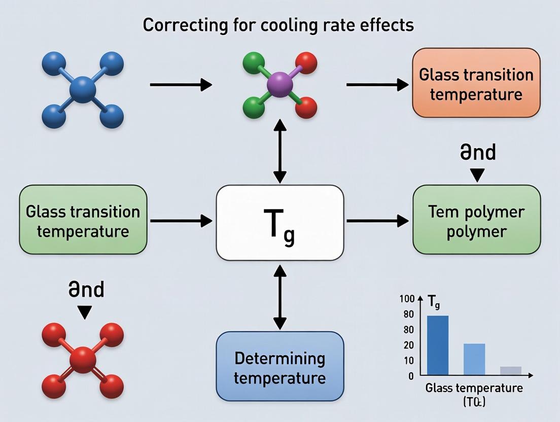
Mastering Tg Analysis: A Comprehensive Guide to Correcting for Cooling Rate Effects in Pharmaceutical Development

Isaac Henderson Jan 12, 2026 245

This article provides a complete framework for researchers and pharmaceutical scientists to understand, quantify, and correct for the significant influence of cooling rate on glass transition temperature (Tg) determination.

Mastering Tg Analysis: A Comprehensive Guide to Correcting for Cooling Rate Effects in Pharmaceutical Development

Abstract

This article provides a complete framework for researchers and pharmaceutical scientists to understand, quantify, and correct for the significant influence of cooling rate on glass transition temperature (Tg) determination. We explore the fundamental kinetic and thermodynamic principles behind the cooling rate dependence, detail established and emerging correction methodologies including annealing protocols and predictive models, and offer best practices for troubleshooting common DSC measurement challenges. A comparative analysis of validation strategies ensures reliable, standardized Tg data critical for predicting amorphous drug stability, optimizing lyophilization cycles, and ensuring product shelf-life in solid dispersions and biologics.

Why Cooling Rate Matters: The Kinetic Nature of Tg and Its Impact on Amorphous Materials

Technical Support Center

Troubleshooting Guides & FAQs

Q1: My measured Tg value for the same polymeric drug formulation shifts between experimental runs. What is the most likely cause? A: This is a classic symptom of uncontrolled cooling rate effects. The glass transition is a kinetics-influenced phenomenon, not an equilibrium thermodynamic event. A faster cooling rate through the transition region results in a higher measured Tg, as the material has less time to relax into a more dense, stable glass. To correct, you must either standardize your cooling protocol precisely or apply a cooling rate correction model.

Q2: When performing DSC, what specific settings are critical for reproducible Tg determination? A: Focus on these parameters:

Cooling/Heating Rate: This is the most critical variable. Always document it precisely (e.g., 10 K/min). For correction studies, multiple rates (e.g., 5, 10, 20, 40 K/min) are required.
Sample Mass: Use small, hermetically sealed pans (3-10 mg) to ensure uniform thermal contact and minimize thermal lag.
Atmosphere: Use inert gas purge (N₂) at a constant flow rate (e.g., 50 ml/min).
Data Analysis Method: Consistently apply the same inflection point (mid-point) or half-step height method for onset determination across all datasets.

Q3: How do I quantitatively correct my Tg data for different cooling rates? A: Apply the Moynihan/Method of Reduced Variables or the Bååth-Arrhenius approach. The core principle is that the structural relaxation time (τ) obeys a Vogel-Fulcher-Tammann (VFT)-type dependence. By performing experiments at multiple cooling rates (q), you can extrapolate to an "equilibrium" Tg at a theoretical cooling rate of zero. See the Experimental Protocol below and the summarized data table.

Q4: In amorphous solid dispersion formulation, why is understanding cooling rate correction crucial? A: The "true" stability and performance metrics (molecular mobility, crystallization tendency, chemical stability) are intrinsically linked to the material's state relative to its equilibrium glass transition. An uncorrected Tg measured at a single, arbitrary cooling rate provides an incomplete picture. Correcting for cooling rate allows for more accurate prediction of long-term storage stability and meaningful comparison between materials processed under different conditions (e.g., spray drying vs. hot-melt extrusion).

Experimental Protocol: Cooling Rate Correction for Tg Determination

Objective: To determine the equilibrium glass transition temperature (Tg₀) of an amorphous material by correcting for cooling rate effects.

Materials & Equipment:

Differential Scanning Calorimeter (DSC) with precise temperature control and programmable cooling rates.
Hermetic aluminum crucibles with lids.
Microbalance.
Amorphous sample (e.g., a drug-polymer solid dispersion).

Procedure:

Sample Preparation: Pre-dry the sample if necessary. Precisely weigh 5-8 mg of material into a hermetic pan and seal it. Prepare an empty, sealed reference pan.
Thermal History Erasure: Load the sample and reference into the DSC. Equilibrate at a temperature 20°C above the expected Tg. Hold isothermal for 5 minutes to erase any previous thermal history.
Multi-Rate Cooling Experiment: Program the following sequence: a. Cool from the equilibration temperature to 50°C below the expected Tg at a defined rate (q₁, e.g., 5 K/min). b. Immediately heat back to the starting temperature at the same rate (q₁). c. Repeat steps a and b for at least three more distinct cooling/heating rates (q₂, q₃, q₄, e.g., 10, 20, 40 K/min). Always start a new cycle from the erased thermal history state.
Data Acquisition: Record the heat flow during the second heating scan for each cooling rate. The heating scan is analyzed to avoid non-linear effects often present in the cooling curve.

Data Analysis:

For each heating curve, determine the Tg (onset or mid-point) using the instrument's software. Denote these as Tg(q).
Apply the Bååth-Arrhenius Correction: a. Plot ln(q) versus 1/Tg(q) for all cooling rates. b. Perform a linear regression on the data. The equation takes the form: ln(q) = ln(A) - Eₐ/(R * Tg(q)), where Eₐ is an apparent activation energy and R is the gas constant. c. Extrapolate the fitted line to a cooling rate approaching zero (e.g., ln(q) → -∞, or practically, a very small q like 0.1 K/min). The corresponding temperature on the 1/Tg axis is the equilibrium glass transition temperature, Tg₀.

Data Presentation

Table 1: Measured Tg vs. Cooling Rate for Model Amorphous Drug (Indomethacin)

Cooling Rate, q (K/min)	Measured Tg (mid-point, °C)	1/Tg (K⁻¹) * 10³	ln(q)
40	48.2	3.115	3.689
20	46.5	3.129	2.996
10	44.9	3.144	2.303
5	43.3	3.161	1.609
Extrapolated Tg₀ (q→0)	40.1 ± 0.5	3.194	-

Note: Data is illustrative based on published literature trends. The extrapolated Tg₀ represents the kinetic slowdown point at infinitesimally slow cooling.

The Scientist's Toolkit

Table 2: Key Research Reagent Solutions for Tg Studies

Item	Function/Description
Hermetic DSC Crucibles	Sealed aluminum pans to prevent sample dehydration or oxidation during heating/cooling scans, which can drastically alter Tg.
Inert Gas (N₂) Supply	Provides a stable, non-reactive atmosphere in the DSC cell, preventing thermal artifacts from oxidation.
Standard Reference Materials	Certified materials (e.g., Indium, Zinc) for temperature and enthalpy calibration of the DSC instrument.
Amorphous Model Compounds	Well-characterized materials like sorbitol, indomethacin, or polymers (PS, PMMA) for method validation and system suitability checks.
Molecular Desiccants	For pre-drying hygroscopic samples (common in pharmaceuticals), as water is a potent plasticizer that lowers Tg.
Thermal Analysis Software	Advanced software capable of performing inflection point analysis and custom fitting routines (e.g., VFT, Arrhenius) for cooling rate correction.

Mandatory Visualization

Diagram Title: Experimental Workflow for Tg Cooling Rate Correction

Technical Support Center: Troubleshooting Tg Determination

Frequently Asked Questions (FAQs)

Q1: Why do I observe a systematic shift in my measured Tg to higher temperatures when I increase the cooling rate during sample preparation for DSC? A: This is the core manifestation of the thermo-kinetic principle. The glass transition is not an equilibrium thermodynamic transition but a kinetic event. At faster cooling rates, the supercooled liquid has less time for molecular rearrangement and configurational relaxation. Therefore, it falls out of equilibrium at a higher temperature, resulting in an elevated Tg. This is an intrinsic property, not an instrument error.

Q2: My DSC data shows an excessively broad Tg step change or multiple inflections. What could be the cause? A: This often indicates non-uniform thermal history or sample issues.

Primary Cause: Inconsistent cooling rate during the initial sample vitrification step. Ensure your DSC cooling program has a controlled, reproducible ramp and is not affected by external drafts or oven door openings.
Secondary Causes: Sample heterogeneity (e.g., phase separation, residual solvents, or uneven powder packing in the pan). Ensure sample preparation is consistent and the pan is hermetically sealed.

Q3: How can I determine if my measured Tg is "rate-independent" or representative of the material's equilibrium properties? A: You cannot from a single measurement. You must perform a series of experiments at different cooling rates (q-) and heating rates (q+). Extrapolation to a rate of zero K/min via established models (like the Vogel–Fulcher–Tammann equation or Moynihan's method) provides an estimate of the equilibrium Tg (Tg0). See Protocol 1 below.

Q4: When performing the heating rate extrapolation method, my data is not linear according to the Lasocka or Moynihan plots. What does this mean? A: Non-linearity in plots of Tg vs. log(q) can indicate:

Insufficient data range: Your range of measured rates may be too narrow. Extend to slower rates if instrumentally possible.
Sample degradation: At slower heating rates, the sample spends more time at elevated temperatures and may degrade, altering the Tg.
Complex underlying kinetics: The material may have distributed relaxation times or competing physical processes (like crystallization during heating). Review your thermograms for overlapping events.

Troubleshooting Guides

Issue: Poor Reproducibility of Tg Between Replicate Runs

Step	Check	Action
1	Sample Mass & Pan	Use identical, hermetically sealed pans. Keep sample mass consistent (±0.2 mg). Large mass causes thermal lag.
2	Instrument Calibration	Re-calibrate temperature and enthalpy using indium and zinc standards at the heating/cooling rates used in your protocol.
3	Thermal History Erasure	Ensure a complete, standardized thermal history erasure cycle (heat above Tg, hold, cool at defined rate) is run before each measurement.
4	Gas Flow & Oven	Maintain identical, stable purge gas flow (typically N2 at 50 ml/min). Check for oven drafts or sensor issues.

Issue: Inconsistent Results When Comparing Data from Different DSC Instruments

Factor	Consideration	Resolution
Furnace Geometry & Sensor	Different thermal lag characteristics.	Perform calibration with standard materials (e.g., polystyrene) across the rate range. Apply instrument-specific lag corrections if software allows.
Cooling Rate Accuracy	The setpoint cooling rate may differ from the actual sample cooling rate.	Validate cooling performance with a blank pan and internal thermocouple check. Always report the programmed rate.
Tg Analysis Method	Different definitions (midpoint, inflection, onset).	Re-analyze all data using the same mathematical definition (e.g., midpoint of the heat flow step change) for comparison.

Experimental Protocols

Protocol 1: Determining the Equilibrium Tg (Tg0) via Cooling Rate Extrapolation

Objective: To correct for the kinetic effect of cooling rate and estimate the equilibrium glass transition temperature.
Materials: See "Research Reagent Solutions" below.
Method:
- Prepare identical, hermetically sealed sample pans.
- Erase thermal history by heating to Tg + 50°C, hold for 5 min.
- Cool the sample from the equilibrium melt to well below Tg at a controlled rate (q-). Use at least 5 different rates (e.g., 1, 2, 5, 10, 20 K/min).
- Immediately heat the sample at a fixed, standard rate (e.g., 10 K/min) through the Tg region to record the thermal response.
- Determine the Tg for each cooling rate using the midpoint method.
- Plot Tg versus the logarithm of the cooling rate (log q-).
- Fit the data linearly and extrapolate to log(q-) → 0 (q- = 1 K/min on a log scale, representing an infinitely slow process) to obtain Tg0.

Protocol 2: Validating the Tool-Narayanaswamy-Moynihan (TNM) Model Parameters

Objective: To characterize the structural relaxation kinetics of a glass-forming system.
Method:
- Perform a series of DSC experiments involving specific thermal histories: (i) Cool from equilibrium at a fixed rate. (ii) Anneal at a temperature below Tg for varying times (ta). (iii) Heat at a fixed rate to observe the enthalpy recovery peak.
- Measure the enthalpy peak position and shape as a function of annealing time and temperature.
- Analyze using TNM equations to solve for the apparent activation energy (Δh*), the non-linearity parameter (x), and the distribution parameter (β). These parameters quantify the rate-dependence.

Data Presentation

Table 1: Exemplar Tg Data for Amorphous Sucrose at Different Cooling Rates (q-) Heating rate (q+) constant at 10 K/min. Data is illustrative.

Cooling Rate, q- (K/min)	Midpoint Tg (°C)	Tg Onset (°C)	Tg Endset (°C)	Step Change ΔCp (J/g·K)
1	62.5	59.1	65.8	0.48
2	63.8	60.3	67.2	0.47
5	65.9	62.1	69.6	0.46
10	68.3	64.5	72.0	0.45
20	71.1	67.0	75.1	0.44

Table 2: Key TNM Model Parameters for Common Pharmaceutical Glass-Formers

Material	Tg0 (K)	Δh* (kJ/mol)	x (Non-linearity)	β (KWW exponent)	Reference Model Fit (R²)
Indomethacin	315	450	0.45	0.65	>0.99
Sucrose	335	600	0.40	0.50	0.98
Trehalose	388	750	0.35	0.45	0.97
PVP K30	448	300	0.55	0.70	>0.99

Visualizations

Title: Kinetic Pathway of Glass Formation & Tg Measurement

Title: TNM Model Structure & Key Parameters

The Scientist's Toolkit: Research Reagent Solutions

Item	Function in Tg Rate-Dependency Studies
Hermetic Aluminum DSC Pans & Lids	Ensures no mass loss (e.g., solvent, decomposition) during heating/cooling scans, critical for precise thermal history control.
Standard Reference Materials (Indium, Zinc, Sapphire)	For calibration of temperature, enthalpy, and heat capacity of the DSC instrument across a range of heating/cooling rates.
Ultra-Pure Inert Gas (N₂, 99.999%)	Provides stable, dry purge atmosphere in the DSC cell, preventing oxidation and condensation during sub-ambient cooling.
Model Glass-Formers (e.g., Sorbitol, Glycerol, Polystyrene)	Well-characterized materials with published TNM parameters, used for method validation and instrument performance checks.
Controlled-Rate Cooling Accessory (Intracooler/LN₂)	Enables precise and reproducible linear cooling at rates from 0.1 to 100+ K/min, essential for q- variation studies.
Non-Linear Regression Software (e.g., Origin, MATLAB with custom scripts)	Required for fitting complex TNM or VFT models to experimental Tg vs. rate data to extract kinetic parameters.

Technical Support Center: Troubleshooting Tg Determination

FAQs & Troubleshooting Guides

Q1: Why does my measured Tg value increase with a faster cooling rate, contradicting some literature? A: This is a common instrumentation artifact. Faster cooling can induce thermal lag, where the sample interior is hotter than the sensor reading. The apparatus registers a transition at an erroneously high temperature.

Troubleshoot: Validate furnace/sample chamber uniformity. Use a smaller sample mass or a sample geometry with higher surface-area-to-volume ratio. Ensure the DSC cell is calibrated for the specific heating/cooling rate range used.

Q2: How can I minimize structural relaxation during the cooling segment before the Tg measurement scan? A: Structural relaxation is inherent but manageable. The goal is to achieve a reproducible, well-defined initial glassy state.

Protocol: Implement a standardized "annealing" protocol above Tg before cooling. For example: Heat to Tg + 30°C, hold isothermally for 10 minutes to erase thermal history, then cool at the specified, controlled rate using a liquid nitrogen cooling accessory or intracooler for maximum control.

Q3: My amorphous material shows enthalpy recovery peaks that obscure the Tg inflection. How do I correct for this? A: Enthalpy recovery peaks indicate substantial relaxation during cooling. They can be minimized or accounted for.

Methodology: Use a "step-scan" or "temperature-modulated DSC (MDSC)" method. The underlying heating rate measures the total heat flow, while the modulated signal deconvolutes it into reversing (heat capacity-related, showing Tg) and non-reversing (relaxation/enthalpy recovery) components. This directly isolates the Tg event.

Q4: What is the quantitative relationship between cooling rate (q_c) and Tg, and how can I use it for correction? A: The relationship is described by the Tool-Narayanaswamy-Moynihan (TNM) model. A common empirical form is: Tg = A + B * log10(|q_c|) where A and B are material-specific constants.

Experimental Protocol to Determine Correction:
- Prepare identical amorphous samples.
- Using a DSC, subject each to a different controlled cooling rate (e.g., 0.5, 1, 2, 5, 10, 20 K/min) from above Tg to well below it.
- Immediately reheat each at a single, standard rate (e.g., 10 K/min) to measure Tg (onset or midpoint).
- Plot Tg vs. log10(|q_c|). Perform linear regression to obtain A and B.
- Correction: To report a standardized Tg, extrapolate/interpolate using this equation to a reference cooling rate (e.g., 10 K/min).

Q5: How does free volume quantitatively change with cooling rate, and how can it be measured? A: Faster cooling traps more excess free volume. This can be characterized via Positron Annihilation Lifetime Spectroscopy (PALS).

PALS Experimental Protocol Summary:
- A positron source (e.g., ²²Na) is placed between two identical glassy sample disks.
- Emitted positrons annihilate with electrons. The lifetime of ortho-positronium (o-Ps) is inversely related to free volume hole size.
- Measure o-Ps lifetime (τ₃) and intensity (I₃) for samples prepared at different cooling rates.
- Calculate mean free volume hole radius (R) using the Tao-Eldrup model: τ₃ = 0.5 [1 - R/(R+ΔR) + (1/2π) sin(2πR/(R+ΔR))]⁻¹, where ΔR is an empirical constant (typically 0.1656 nm).

Table 1: Effect of Cooling Rate on Tg for Model Polymer (Polystyrene)

Cooling Rate, q_c (K/min)	Tg (Midpoint) (°C)	Tg (Onset) (°C)	Enthalpy Recovery Peak Area (J/g)
1	99.5	96.2	0.8
5	100.8	97.5	1.5
10	101.5	98.1	2.1
20	102.3	98.9	3.0
40	103.1	99.6	4.2

Table 2: PALS Free Volume Data for Amorphous Drug (Indomethacin)

Cooling Rate (K/min)	o-Ps Lifetime, τ₃ (ns)	Free Volume Hole Radius, R (Å)	Relative Free Volume Fraction (I₃ * R³)
2	1.82	2.64	1.00 (normalized)
10	1.88	2.69	1.12
Quenched (~50)	1.94	2.74	1.25

Experimental Workflow & Conceptual Diagrams

Workflow for Tg vs Cooling Rate Experiment

Physical Basis of Cooling Rate Effect

The Scientist's Toolkit: Research Reagent Solutions

Table 3: Essential Materials for Cooling Rate Studies

Item	Function & Rationale
DSC with Intracooler	Provides precise, controlled cooling rates from slow (0.1 K/min) to fast (50+ K/min) for reproducible thermal history creation.
Hermetic Sealed DSC Pans	Prevents sample degradation or moisture loss during prolonged holds above Tg and ensures consistent thermal contact.
Liquid Nitrogen Cooling Accessory	Enables rapid quench cooling for creating high free volume glasses, extending the range of studied q_c.
Temperature-Modulated DSC Software	Deconvolutes total heat flow to isolate the glass transition from overlapping enthalpy recovery events.
Standard Reference Materials (e.g., Indium, Tin)	Essential for calibration of temperature and enthalpy across the entire heating and cooling rate range used.
Gas Quenching Device	For bulk sample preparation, allows rapid cooling of films or powders in a controlled atmosphere for subsequent PALS or stability studies.
Positron Annihilation Lifetime Spectrometer	Directly measures free volume hole size and distribution in the glassy state as a function of cooling history.

Technical Support Center

Troubleshooting Guide & FAQs

Q1: During lyophilization cycle development, our amorphous protein formulation consistently collapses. How does the measured Tg' relate to this, and how can we prevent it? A: Collapse occurs when the product temperature exceeds the collapse temperature (Tc), often closely related to the glass transition temperature of the maximally freeze-concentrated solute (Tg'). Tc is typically a few degrees above Tg'. To prevent collapse:

Ensure primary drying is conducted at a shelf temperature that keeps the product temperature at least 2-3°C below the experimentally determined Tg'.
Use a conservative cycle with lower shelf temperature and longer duration.
Consider formulation optimization with stabilizers (e.g., disaccharides) that elevate Tg'.

Q2: Our API solution shows unpredictable crystallization during freeze-thaw or lyophilization. How can we assess this risk from thermal data? A: Unwanted crystallization is often due to insufficient cooling rates or annealing steps that promote crystalline hydrate formation. Assess risk using:

Differential Scanning Calorimetry (DSC): Look for recrystallization exotherms during warming of a quickly cooled sample. The absence of a Tg' can indicate crystallization.
Protocol: Quench-cool the solution in the DSC (e.g., 50°C/min) to -60°C, then warm at 2-5°C/min. Analyze for Tg' and crystallization events.
Solution: Optimize the cooling rate or include an annealing step above Tg' but below the melting point to drive controlled crystallization if a stable crystalline form is desired.

Q3: Why do we get different Tg' values for the same formulation when using different DSC instruments or cooling rates, and how do we correct for this? A: Tg' is a non-equilibrium state. Measured values are kinetically controlled and depend on the thermal history (cooling rate). Faster cooling can lead to a higher apparent Tg' due to incomplete freeze-concentration.

Correction Protocol: Perform a "cooling rate dependence" study.
- Prepare identical samples.
- Run DSC cycles with varying cooling rates (e.g., 1, 5, 10, 20°C/min) from room temperature to -60°C.
- Warm all samples at the same standard rate (e.g., 5°C/min).
- Plot the measured Tg' versus cooling rate. Extrapolate to a "zero cooling rate" to estimate the theoretical Tg' at equilibrium.
Solution: Standardize the cooling rate protocol within your lab. For critical comparisons, report the cooling rate used and consider the extrapolated value.

Q4: After lyophilization, our product shows poor reconstitution time. What formulation or process factors related to Tg are likely causes? A: Poor reconstitution is often linked to excessive collapse or high residual moisture, which can be traced to Tg.

Cause 1: Collapse (product temp > Tg'/Tc) creates a dense, impermeable cake.
Cause 2: High residual moisture plasticizes the amorphous solid, lowering the glass transition temperature of the dry cake (Tg). If storage temperature exceeds this lowered Tg, micro-collapse and pore closure can occur.
Troubleshooting: Ensure complete secondary drying. Measure the Tg of the final cake via DSC. Ensure storage temperature is well below (e.g., ≥50°C below) the product's Tg to maintain cake structure.

Table 1: Impact of Cooling Rate on Measured Tg' for a Model mAb-Sucrose Formulation

Cooling Rate (°C/min)	Measured Tg' (°C)	Onset of Recrystallization Exotherm (°C)
1	-41.2 ± 0.5	-33.5 ± 0.8
5	-39.8 ± 0.4	-35.1 ± 0.6
10	-38.5 ± 0.6	-36.8 ± 0.5
20	-37.1 ± 0.7	Not Observed
Extrapolated to 0°C/min	-42.5 ± 0.9	-

Table 2: Effect of Stabilizer on Thermal Properties and Lyophilization Outcome

Formulation (5 mg/mL mAb)	Tg' (°C)	Tc (by FDM*) (°C)	Cake Appearance (at -40°C Shelf)	Reconstitution Time (s)
Sucrose (60 mg/mL)	-39.8	-37	Elegant, porous	12 ± 2
Trehalose (60 mg/mL)	-40.5	-38	Elegant, porous	10 ± 3
No Stabilizer	-28.1 (broad)	-27	Severe Collapse	>300

*Freeze-Dry Microscopy

Experimental Protocols

Protocol 1: Determining Tg' with Cooling Rate Correction Objective: To obtain a reproducible, cooling-rate-corrected Tg' value for formulation development. Materials: See "The Scientist's Toolkit" below. Method:

Load 10-30 µL of formulation into a Tzero Hermetic DSC pan. Seal crucible.
Equilibrate at 25°C for 2 min.
Cool to -60°C at a defined rate (e.g., 5°C/min). Note: This is the critical variable.
Hold isothermally at -60°C for 5 min.
Warm to 10°C at a standard rate of 5°C/min.
Analyze the warming curve. Tg' is identified as the midpoint of the step change in heat capacity.
Repeat steps 1-6 for at least 3 different cooling rates (e.g., 1, 10, 20°C/min).
Plot Tg' (y-axis) vs. Cooling Rate (x-axis). Perform linear regression and extrapolate to a cooling rate of 0°C/min to estimate the equilibrium Tg'.

Protocol 2: Freeze-Dry Microscopy (FDM) for Collapse Temperature (Tc) Objective: Visually determine the collapse temperature of a formulation. Method:

Place a small droplet (~2 µL) of the formulation on a temperature-controlled FDM stage.
Rapidly freeze the sample to -50°C.
Apply vacuum to the stage chamber to simulate primary drying.
Warm the stage slowly (e.g., 2°C/min) while observing under polarized light.
Record the temperature at which the microstructure of the frozen sample begins to lose porosity and visibly flow/viscously collapse. This is the Tc.
The primary drying shelf temperature should be set 2-5°C below this Tc.

Diagrams

Cooling Path Impact on Final Product State

Workflow: Correcting Tg' for Robust Lyophilization

The Scientist's Toolkit: Key Research Reagent Solutions

Item	Function in Tg'/Lyophilization Research
Tzero Hermetic DSC Pans & Lids	Ensures a sealed, non-leaking environment for analyzing aqueous formulations during temperature ramps.
High-Resistance DSC Instrument	Provides the sensitivity needed to detect the subtle heat capacity changes at Tg' in dilute biopharmaceutical solutions.
Freeze-Dry Microscope (FDM)	Allows direct visualization of collapse, meltback, and crystallization events in real-time under vacuum and temperature control.
Lyophilization Stabilizers(e.g., Sucrose, Trehalose)	Amorphous excipients that raise Tg', vitrify the API, and provide a stable hydrogen-bonding matrix in the dry state.
Thermal Analysis Software	Used for complex analysis of DSC data, including step-change quantification and kinetics of thermal events.
Controlled Ice Nucleation Agent(e.g., based on inert gas pressure shift)	Promotes uniform ice crystal structure, reducing inter-vial heterogeneity and improving drying consistency.

Key Literature and Landmark Studies on Cooling Rate Dependence

This technical support center provides troubleshooting guidance for researchers working on correcting cooling rate effects in glass transition temperature (T_g) determination, a critical parameter in amorphous solid dispersion and biopharmaceutical formulation stability.

Frequently Asked Questions (FAQs) & Troubleshooting

Q1: Why does my measured T_g value increase with faster cooling rates in DSC experiments, contradicting some literature? A: This is a common instrumentation artifact. At very high cooling rates, the DSC furnace may not be in perfect thermal equilibrium with the sample, leading to a lag and an apparent higher T_g. Troubleshooting Steps:

Verify Calibration: Perform a heating rate and cooling rate calibration using standard materials (e.g., Indium for heating, specific organic standards for cooling).
Reduce Sample Mass: Use sample masses ≤ 5 mg to improve thermal contact and reduce thermal lag.
Validate Rate: Repeat the experiment at a moderately slow cooling rate (e.g., 5-10 K/min). The established trend should be a decrease in T_g with increased cooling rate due to thermodynamics.

Q2: How do I correct for cooling rate effects to report a standardized T_g? A: The most cited method is to use the Moynihan / ASTM E1356 protocol. You must perform multiple DSC runs. Experimental Protocol:

Prepare identical samples (same mass, pan type, packing).
Run DSC cycles: Heat above T_g → Hold to erase thermal history → Cool at a specific rate (β_c: e.g., 40, 20, 10, 5 K/min) → Reheat at a fixed rate (β_h: e.g., 10 K/min) to measure T_g.
Plot the measured T_g against the logarithm of the cooling rate (log β_c).
Fit the data linearly. Extrapolate to a log β_c of zero (i.e., an infinitely slow cooling rate) to obtain the standardized T_g.

Q3: My T_g versus cooling rate plot is non-linear. What does this indicate? A: Non-linearity, especially at very slow or very fast cooling rates, often indicates:

Sample Degradation: Slow cooling allows more time for chemical or physical change.
Crystallization/Relaxation: The sample may be crystallizing or undergoing significant structural relaxation during the slow cool.
Instrument Limitation: At very fast rates, the furnace response is non-ideal. Troubleshooting: Characterize post-run samples via XRPD or microscopy to check for crystallization. Use modulated-temperature DSC (MTDSC) to deconvolve reversing and non-reversing heat flows.

Q4: How does moisture affect cooling rate dependence studies? A: Moisture is a potent plasticizer that drastically lowers T_g and alters kinetics. Its effect interacts with cooling rate.

Issue: An incompletely dried sample will show an anomalously low T_g and exaggerated cooling rate dependence.
Solution: Implement rigorous drying protocols prior to analysis (e.g., vacuum drying, P₂O₅ desiccation) and use hermetically sealed pans. Consider using TGA-coupled methods to confirm dryness.

Key Data from Landmark Studies

Table 1: Summary of Cooling Rate Effects on T_g for Model Pharmaceuticals

Material/System	Cooling Rates Tested (K/min)	Extrapolated T_g at β→0 (°C)	Apparent Activation Energy (Δh*/R)	Key Finding	Primary Citation
Pure Amorphous Sucrose	0.5 – 30	~67	~ 800 K	Demonstrated classic Moynihan behavior; established protocol for pharmaceuticals.	Bhugra et al., J Pharm Sci, 2008.
Indomethacin-PVP VA64 Dispersion	5 – 40	~113.5	Varies with comp.	Cooling rate dependence weakens with increasing polymer content; critical for predicting stability.	Kothari et al., Mol Pharm, 2015.
Spray-Dried Protein (mAb)	1 – 20	~144	~ 650 K	Showed cooling rate effects are critical for accurate T_g determination in biologics, impacting shelf-life.	Mensink et al., Eur J Pharm Biopharm, 2017.
Annealed Trehalose	2 – 50	~80 (for annealed)	N/A	Annealing near T_g reduces cooling rate dependence, indicating a more "equilibrated" glass.	Zhou et al., Thermochim Acta, 2019.

Table 2: Standardized Experimental Protocol for Cooling Rate Correction

Step	Action	Critical Parameters	Purpose
1. Sample Prep	Dry, powder homogenization.	Use ≤ 5 mg; hermetically sealed pan.	Minimize thermal lag and moisture.
2. Thermal History Erasure	Heat to T_g + 30°C, hold 3-5 min.	Must be above T_g but below decomp.	Creates uniform starting structure.
3. Controlled Cooling	Cool at target rate (β_c) to T_g - 50°C.	At least 4 different rates (e.g., 40,20,10,5).	Generates glasses with different fictive temps.
4. T_g Measurement	Reheat at fixed rate (β_h, e.g., 10 K/min).	Midpoint or inflection method must be consistent.	Measures T_g as function of β_c.
5. Data Analysis	Plot T_g vs. log β_c; linear extrapolation to log β_c=0.	Use linear regression; report R².	Obtains cooling-rate-independent T_g.

Visualization of Protocols and Relationships

Experimental Workflow for Cooling Rate Correction

Logical Relationship of Cooling Rate to Tg and Stability

The Scientist's Toolkit: Essential Research Reagents & Materials

Table 3: Key Research Reagent Solutions for Cooling Rate Studies

Item	Function/Brief Explanation	Example/Note
Hermetic Sealed DSC Pans (Aluminum)	Ensures no mass loss (moisture, solvent) during heating/cooling cycles, critical for accurate thermal data.	Use with sealing press; ensure crimp is tight.
High-Purity Inert Standard (e.g., Sapphire)	Used for calibration of DSC heat capacity, necessary for quantitative comparison of Cp jumps at T_g.	NIST-traceable standard recommended.
Cooling Rate Calibration Standard	Organic materials with known melting points used to verify the true cooling rate of the DSC furnace.	e.g., Biphenyl, Naphthalene.
Desiccant (e.g., P₂O₅)	For rigorous drying of samples and storage in desiccators to eliminate plasticizing effects of moisture.	Use in vacuum desiccator; handle with care.
Thermal Analysis Software	Enables advanced data analysis: curve fitting, derivative plots, and linear extrapolation of Tg vs. log βc.	Often instrument-specific (TA, Mettler, PerkinElmer).
Modulated DSC (MDSC) Capability	Allows separation of reversing (heat capacity) and non-reversing (relaxation, crystallization) events, clarifying complex data.	Not a reagent, but a critical instrumental method.

From Theory to Practice: Methodologies for Measuring and Correcting Cooling Rate Effects

Standardized DSC Protocols for Consistent Tg Measurement

Technical Support & Troubleshooting Center

FAQ 1: Why do I get different Tg values when I repeat the measurement on the same polymer sample?

Answer: Inconsistent Tg values often stem from variations in the sample's thermal history. If the sample is not subjected to a controlled, standardized thermal protocol (specific heating/cooling rates, hold times) before measurement, its physical state will differ. This directly impacts the enthalpy relaxation and the resulting Tg. Within the thesis context, this highlights the critical need for a standardized pre-Tg conditioning protocol to erase variable thermal histories before applying the cooling-rate correction.

FAQ 2: How does the DSC cooling rate affect the measured Tg, and how can I correct for it?

Answer: The cooling rate during the vitrification step prior to Tg measurement has a pronounced effect. Faster cooling rates result in a higher measured Tg because the polymer has less time to relax into a more stable configuration. The correction is a core focus of the associated thesis. A methodology involves measuring Tg at multiple, controlled cooling rates (e.g., 1, 5, 10, 20 K/min) and extrapolating to a Tg at 0 K/min (equilibrium cooling) using an established model like the Vogel–Fulcher–Tammann (VFT) equation or Tool-Narayanaswamy-Moynihan (TNM) formalism.

FAQ 3: My DSC baseline shows significant drift or instability around Tg. What could be the cause?

Answer: Baseline issues can arise from: 1) Poor sample-pan contact: Ensure the sample pan is clean, crimped properly, and sits flat in the sample holder. 2) Sample mass too large: Use a sample mass appropriate for your DSC cell (typically 5-15 mg for polymers). 3) Purge gas flow rate fluctuations: Verify and stabilize the nitrogen purge gas flow (usually 50 mL/min). 4) Contamination: Clean the sensor/furnace if previous samples decomposed.

FAQ 4: What is the best way to determine the onset, midpoint, and endpoint Tg from a DSC curve?

Answer: Consistency in Tg assignment is as important as the measurement itself. Use the following step-by-step protocol on the re-heating scan after controlled cooling:
- Baseline Drawing: Draw a straight baseline from the region well below the transition (e.g., 30°C below onset) to the region well above (e.g., 30°C above endpoint).
- Step Determination: Identify the step change in heat capacity (ΔCp).
- Onset (Tg-onset): Extrapolate the baseline before the transition and the steepest tangent of the step. The intersection is Tg-onset.
- Midpoint (Tg-mid): The temperature at which half of the ΔCp step change has occurred.
- Endpoint (Tg-end): Extrapolate the baseline after the transition and the steepest tangent of the step. The intersection is Tg-end. Report which method (onset/midpoint) is used.

Experimental Protocols

Protocol 1: Standardized Sample Preparation & Conditioning for Tg Measurement

Drying: Dry the sample in a vacuum oven at a temperature at least 20°C below its estimated Tg for 24 hours to remove moisture.
Encapsulation: Weigh 5-10 mg (±0.01 mg) of material into a hermetically sealed aluminum DSC pan. Use an empty, identical pan as a reference.
Thermal History Erasure: Load the sample into the DSC and run the following conditioning program:
- Heat from 25°C to Tgest + 30°C at 10 K/min.
- Hold isothermally for 5 minutes to erase thermal history.
- Critical Cooling Step: Cool to Tgest - 50°C at a precisely controlled, documented rate (e.g., 10 K/min). This rate becomes a key variable for correction.
- Hold for 2 minutes at the lower temperature.
Measurement Scan: Re-heat the sample to Tgest + 30°C at a standard rate of 10 K/min. Record this heat flow curve for initial Tg analysis.

Protocol 2: Determining Cooling Rate Dependence & Correcting to Equilibrium Tg

Perform Protocol 1 repeatedly on identical sample aliquots, but systematically vary the Critical Cooling Step rate (β_cool). Use at least four rates (e.g., 1, 2, 5, 10, 20 K/min).
For each cooling rate, record the subsequent reheating curve and determine the Tg (midpoint method recommended for consistency).
Tabulate Cooling Rate (K/min) vs. Measured Tg (°C).
Data Fitting: Plot Tg against cooling rate. Fit the data to the Vogel–Fulcher–Tammann (VFT) type equation for Tg dependence: T_g(β) = T_g0 + A / (log(β) - B) where T_g0 is the extrapolated equilibrium glass transition temperature at 0 K/min cooling rate, and A, B are fitting parameters.
The fitted parameter T_g0 represents the cooling-rate-corrected, equilibrium Tg.

Data Presentation

Table 1: Effect of Controlled Cooling Rate on Measured Tg for Amorphous Polymer X

Sample Aliquot	Controlled Cooling Rate (β), K/min	Measured Tg (Midpoint), °C	ΔCp, J/(g·K)
A1	1.0	72.5	0.352
A2	2.0	73.8	0.348
A3	5.0	75.6	0.345
A4	10.0	77.2	0.341
A5	20.0	79.1	0.337

Table 2: VFT Model Fitting Parameters from Data in Table 1

Fitted Parameter	Value	Description
T_g0	70.2 ± 0.3 °C	Extrapolated Tg at 0 K/min (Equilibrium Tg)
A	525.7 K	VFT fitting constant
B	-1.89	VFT fitting constant
R²	0.998	Goodness of fit

Visualization: Workflow & Relationship Diagrams

Workflow for Cooling Rate Correction in Tg Measurement

Logical Relationship: From Problem to Corrected Solution

The Scientist's Toolkit: Research Reagent Solutions

Table 3: Essential Materials for Standardized DSC Tg Experiments

Item	Function & Importance
Hermetically Sealed Aluminum DSC Pans & Lids	Ensures no mass loss or contamination during heating/cooling cycles. Critical for stable baseline.
High-Purity Nitrogen Gas (≥99.999%)	Inert purge gas to prevent oxidative degradation of samples at high temperatures.
Calibrated Standard (Indium, Zinc)	Used for temperature and enthalpy calibration of the DSC instrument, ensuring accuracy.
Microbalance (0.01 mg readability)	Accurate sample weighing (5-10 mg) is essential for reproducible heat capacity measurements.
Vacuum Oven	For thorough drying of samples to eliminate water plasticization, which significantly lowers Tg.
Thermal Analysis Software with Advanced Kinetics Module	Enables fitting of Tg(β) data to VFT/TNM models for equilibrium Tg extrapolation.

Troubleshooting Guide & FAQs

Q1: After annealing, my subsequent DSC scan still shows an enthalpy relaxation peak near the Tg. What went wrong? A1: This indicates incomplete erasure of the thermal history. The likely cause is insufficient annealing time at the chosen temperature. Ensure the annealing duration is significantly longer than the material's characteristic relaxation time at that temperature. For polymeric systems, a common rule is to anneal for at least 3-5 times the estimated τ (relaxation time) of the α-process. Verify that your annealing temperature (Ta) is within the correct range, typically Tg - 10°C to Tg + 20°C for most organic glasses. Also, confirm that your cooling rate from the annealing temperature to below Tg was sufficiently slow (e.g., 0.5-2°C/min) to avoid reintroducing non-equilibrium structure.

Q2: How do I determine the optimal annealing temperature and time for my novel amorphous solid dispersion? A2: There is no universal setting. You must perform a preliminary characterization.

Run an initial fast DSC scan (e.g., 20°C/min) to get an approximate Tg.
Design a temperature-time matrix experiment. Anneal multiple samples at different temperatures (e.g., Tg-15, Tg-5, Tg+5, Tg+15°C) for varying times (e.g., 30 min, 2 hrs, 8 hrs).
Analyze the enthalpy recovery. After each annealing protocol, cool the sample at a controlled rate (e.g., 10°C/min) and then rescan in the DSC. The sample with the smallest (or absent) enthalpy relaxation peak in the second scan represents the most effective annealing conditions for erasing prior history. See Table 1 for example results.

Q3: My material crystallizes during the annealing step intended to erase thermal history. How can I prevent this? A3: Crystallization during annealing means the material is metastable and your Ta is within or above its crystallization temperature range.

Mitigation Strategy 1: Lower the annealing temperature. Stay significantly below the onset of crystallization (Tx) observed in your initial DSC scan. A safe zone is often between Tg and (Tg + 10°C).
Mitigation Strategy 2: Reduce annealing time. Use shorter annealing periods and check for erasure of the enthalpy peak. You may need to iterate.
Mitigation Strategy 3: Consider using Stepwise Annealing. Instead of one long isothermal hold, use a series of shorter holds at incrementally increasing temperatures below Tx to gradually approach equilibrium without triggering crystallization.

Q4: For correcting cooling rate effects in Tg determination, should I anneal above or below the nominal Tg? A4: For this specific research goal, annealing below the nominal Tg is critical. The objective is to equilibrate the sample into a state corresponding to a specific, slower cooling rate than was actually used. For example, to mimic an infinitely slow cooling rate (theoretical equilibrium glass), you would anneal at a temperature just below the expected equilibrium Tg (typically Tg_infinity) for an extended period (often hours to days). Annealing above Tg creates a liquid state, and subsequent cooling will imprint a new thermal history, which is not the goal when correcting for past cooling rate effects.

Q5: How do I quantitatively relate my annealing protocol to an "equivalent cooling rate" for my Tg correction study? A5: This requires coupling the Tool-Narayanaswamy-Moynihan (TNM) or KAHR model with your annealing data.

Protocol: Perform annealing experiments at several sub-Tg temperatures (Ta).
Measurement: After each anneal, immediately run a DSC scan to measure the endothermic enthalpy recovery peak (ΔH).
Analysis: The value of ΔH is related to the "fictive temperature" (Tf). The annealing process lowers Tf towards Ta. The relationship between annealing time at Ta and the shift in Tf can be modeled to calculate the equivalent cooling rate that would have resulted in that same Tf. This is a non-linear fitting procedure requiring specialized software.

Experimental Protocol: Standard Annealing for Thermal History Erasure

Objective: To erase previous thermal history and achieve a reproducible, well-defined initial glassy state for subsequent Tg measurement.

Materials: Differential Scanning Calorimeter (DSC), hermetic Tzero pans/lids, analytical balance, inert gas (N2).

Procedure:

Sample Preparation: Pre-dry the sample if hygroscopic. Accurately weigh (3-10 mg) into a DSC pan and hermetically seal it.
Initial Erasure Scan: Load the sample and an empty reference pan into the DSC. Purge with N2 (50 mL/min).
- Equilibrate at Tstart = Tg - 50°C.
- Heat at 20°C/min to Terase = Tg + 30°C (or 20°C above any prior thermal event). Hold for 5 minutes. This step melts/erases all prior thermal history.
Controlled Cooling: Cool from Terase to Tanneal = Tg + 10°C at a rate of 50°C/min (to set a controlled "fast" baseline history). Then immediately cool to the chosen Annealing Temperature (Ta). A typical Ta is Tg - 5°C.
Isothermal Anneal: Hold isothermally at Ta for the predetermined annealing time (ta). Common ta ranges from 30 minutes to 8 hours, depending on the material.
Quenching: After the annealing hold, rapidly cool the sample to T_start at the maximum achievable rate of your DSC (e.g., 100-200°C/min). This "freezes in" the annealed structure.
Measurement Scan: Immediately perform the final DSC scan from Tstart to Terase at your standard heating rate (e.g., 10°C/min) to measure the Tg and check for any residual enthalpy relaxation.

Data Analysis: A successful annealing protocol for history erasure will result in a final DSC scan with a clear, single Tg step change in heat capacity, with no (or a minimal) endothermic overshoot preceding it.

Table 1: Example Results from Annealing Temperature/Time Matrix on an Amorphous API (Nominal Tg ≈ 50°C)

Annealing Temp (Ta)	Annealing Time (ta)	Enthalpy Recovery Peak (ΔH, J/g)	Observation
35°C (Tg-15)	2 hours	1.2	Small peak persists
35°C (Tg-15)	8 hours	0.3	Very small peak
45°C (Tg-5)	30 min	2.5	Large peak
45°C (Tg-5)	2 hours	0.8	Moderate peak
55°C (Tg+5)	30 min	0.0	No peak - Optimal
55°C (Tg+5)	2 hours	0.0 (but crystallization)	Crystallization occurred

Table 2: TNM Model Parameters for a Model Polymer (Polycarbonate) for Equivalent Cooling Rate Calculation

Parameter	Symbol	Value	Description
Activation Energy	Δh*/R (K)	~100,000 K	Barrier for structural relaxation
Non-linearity Parameter	x	~0.4	Defines temperature dependence of relaxation times
Structural Parameter	β	~0.5	Stretching exponent (width of relaxation)
Log(Pre-factor)	log(A/s)	~ -150	Arrhenius factor for relaxation time

Diagrams

Thermal History Erasure Workflow for Tg Measurement

Relationship Between Annealing and Equivalent Cooling Rate

The Scientist's Toolkit: Research Reagent Solutions

Table 3: Essential Materials for Annealing & Tg Correction Studies

Item	Function/Description	Critical Specification
High-Precision DSC	Measures heat flow to detect Tg and enthalpy relaxation. Must have excellent baseline stability and sub-ambient capability.	Temperature precision < ±0.1°C; Calibrated with In, Zn, Ga standards.
Hermetic Tzero Pans & Lids	Sealed crucibles to prevent sample loss/degradation and ensure good thermal contact. Essential for volatile or hygroscopic samples.	Aluminum or gold-plated steel. Must be hermetically sealed with a crimper.
Ultra-Pure Inert Gas	Dry nitrogen or argon purge gas to prevent oxidation and condensation in the DSC cell during slow cooling/annealing.	>99.999% purity, with in-line moisture/oxygen trap.
Standard Reference Materials	For calibration (In, Zn, Sapphire) and method validation (e.g., polystyrene with known Tg).	Certified reference materials (CRMs) from NIST or equivalent.
Modeling Software	Software capable of performing TNM/KAHR model fitting to extract relaxation parameters and calculate equivalent cooling rates.	Examples: TA Instruments TRIOS, Netzsch Proteus, or custom MATLAB/Python scripts.
Controlled Humidity Chamber	For preconditioning hygroscopic samples to a specific water content, which significantly affects Tg and relaxation kinetics.	Capable of maintaining ±1% RH stability.
Low-Thermal-Mass Desiccator	For storing annealed samples before measurement if they cannot be tested immediately in the DSC.	Contains dry desiccant (e.g., P2O5) to prevent moisture uptake.

FAQs

Q1: Why is constructing a Tg vs. Log(Cooling Rate) plot critical in my research? A1: This plot is foundational for correcting cooling rate effects in Tg determination. The glass transition temperature (Tg) is kinetic; it shifts to lower values at slower cooling rates. By establishing this relationship, you can extrapolate to find the "equilibrium" Tg at an infinitely slow cooling rate (a theoretical value), allowing for the comparison of materials under standardized conditions, which is vital for robust formulation science in drug development.

Q2: My DSC thermograms show broad or poorly defined Tg steps. What could be the cause? A2: Common causes include:

Insufficient sample quantity: Typically, 5-20 mg is required for amorphous organic materials.
Sample history: Prior thermal or mechanical treatment can affect the enthalpy relaxation peak. Always use a freshly prepared sample or employ a standardized annealing protocol (see protocol below).
Excessive moisture: Hygroscopic pharmaceutical materials can show broad transitions. Dry samples in a desiccator or under dry nitrogen purge before analysis.
Cooling/Heating rate mismatch: For the correction plot, the heating rate for measurement must be constant, while the prior cooling rate is varied.

Q3: How many cooling rates should I investigate for a reliable plot? A3: A minimum of four distinct cooling rates over at least two orders of magnitude (e.g., 1, 5, 10, 20 K/min) is recommended. More data points improve the linear regression fit for the extrapolation.

Q4: What is the acceptable R² value for the linear fit of Tg vs. Log(Cooling Rate)? A4: For reliable extrapolation, aim for an R² value ≥ 0.98. A lower value suggests scatter, possibly due to poor thermal contact, sample degradation, or inconsistent Tg determination method.

Troubleshooting Guides

Issue: Poor Reproducibility Between Replicates

Check 1: Ensure identical sample preparation (mass, packing in the pan). Use hermetically sealed pans to prevent mass loss.
Check 2: Verify the DSC calibration (temperature and enthalpy) using standard references like Indium at the relevant cooling rates.
Check 3: Implement a rigorous thermal history erasure protocol before each experiment (see Standard Protocol below).

Issue: Non-Linear Tg vs. Log(Cooling Rate) Data

Check 1: Confirm the Tg determination method is consistent (midpoint, inflection point) and automated via software to remove user bias.
Check 2: Ensure the sample is fully amorphous. Partial crystallinity can distort the Tg step. Verify by XRPD.
Check 3: Assess for chemical or physical degradation during the repeated thermal cycles. Run a final heating scan and compare to the first.

Experimental Protocols

Standard Protocol for Tg vs. Log(q) Data Collection via DSC

Objective: To collect the Glass Transition Temperature (Tg) of an amorphous pharmaceutical material at multiple controlled cooling rates (q) for extrapolation.

Materials: Differential Scanning Calorimeter (DSC), hermetically sealed aluminum pans, analytical balance, dry nitrogen purge gas.

Procedure:

Sample Preparation: Pre-dry the sample if hygroscopic. Precisely weigh 5-10 mg (± 0.01 mg) into a DSC pan and hermetically seal it.
Instrument Setup: Purge the DSC cell with dry nitrogen (50 ml/min). Allow furnace to equilibrate.
Thermal History Erasure:
- Heat the sample to at least 30°C above its expected Tg (e.g., to T_g + 50°C) at a standard rate (e.g., 20 K/min).
- Hold isothermally for 5 minutes to erase any previous thermal history and allow molecular relaxation.
Controlled Cooling:
- Cool the sample to at least 50°C below the expected Tg at the target cooling rate (q₁). Common rates: 1, 2, 5, 10, 20, 40 K/min.
Tg Measurement Scan:
- Immediately re-heat the sample from the low temperature to above Tg at a fixed heating rate (typically 10 K/min).
- Record the thermogram. Determine Tg using the midpoint method (half-step height) via instrument software.
Replication & Variation:
- Repeat steps 3-5 for the same sample pan using the next cooling rate (q₂, q₃...). Run in triplicate using fresh sample aliquots.
Data Compilation: Tabulate Tg (mean ± SD) against the applied cooling rate (q).

Protocol for Data Analysis and Plot Construction

Calculate Logarithm: For each cooling rate (q in K/min), calculate log₁₀(q).
Plot: On a standard Cartesian plot, place Tg (in °C or K) on the Y-axis and log₁₀(q) on the X-axis.
Linear Regression: Perform a least-squares linear regression: Tg = m * log₁₀(q) + c.
Extrapolation: The y-intercept (c) represents the extrapolated Tg at a cooling rate of 1 K/min (log(1)=0). Further extrapolation to "equilibrium" Tg (Tg₀) requires specific models (e.g., Vogel–Fulcher–Tammann) but a linear fit over a practical range is standard for formulation screening.

Data Presentation

Table 1: Exemplar Data for Amorphous Sucrose Data sourced from recent thermal analysis literature on pharmaceutical sugars.

Cooling Rate, q (K/min)	log₁₀(q)	Tg (midpoint), °C (Mean ± SD, n=3)
40	1.602	64.2 ± 0.5
20	1.301	66.8 ± 0.3
10	1.000	68.5 ± 0.4
5	0.699	70.1 ± 0.6
2	0.301	72.4 ± 0.7
1	0.000	73.9 ± 0.5

Table 2: Linear Regression Parameters from Exemplar Data

Parameter	Value	Description
Slope (m)	-6.47	Sensitivity of Tg to cooling rate (ºC/log)
Intercept (c)	73.9	Extrapolated Tg at q=1 K/min (ºC)
R²	0.994	Goodness of linear fit

Mandatory Visualization

Tg vs Log(q) Data Collection Workflow

Concept of Cooling Rate Extrapolation for Tg

The Scientist's Toolkit

Table 3: Essential Research Reagent Solutions for Tg Correction Studies

Item	Function/Brief Explanation
High-Performance DSC	Essential for precise temperature control and heat flow measurement across a wide range of cooling rates (0.5 to 100+ K/min).
Hermetically Sealed DSC Pans & Lids	Ensure no mass loss or moisture uptake during heating/cooling cycles, critical for reproducibility.
Ultra-Pure Inert Gas (N₂)	Purge gas to prevent oxidation and condensation in the DSC cell during sub-ambient cooling.
Standard Calibration Materials (Indium, Zinc)	Used for temperature and enthalpy calibration at specific cooling/heating rates.
Desiccator & Drying Agent (P₂O₅)	For pre-drying hygroscopic pharmaceutical samples (APIs, polymers) to remove plasticizing water.
Amorphous Model Compound (e.g., Sucrose, Trehalose)	Well-characterized, easily vitrified material for method validation and instrument performance checks.
Statistical Software	For performing linear regression and evaluating the fit of the Tg vs. Log(q) data.

Troubleshooting Guide & FAQs

Q1: What does the Moynihan equation correct for, and when should I use it over the Lasocka equation?

A: The Moynihan equation is used to correct the cooling rate dependence of the glass transition temperature (Tg) measured via Differential Scanning Calorimetry (DSC). It applies a linear regression to data obtained at multiple cooling rates to extrapolate to an equilibrium Tg at a cooling rate of 0 K/min. Use the Moynihan equation when you have data from at least 3-4 different cooling rates and the relationship between Tg and the logarithm of the cooling rate (lnq) is approximately linear.

Q2: My Moynihan plot (Tg vs. ln q) shows significant curvature. What does this mean, and how do I proceed?

A: Significant curvature in a Moynihan plot indicates a breakdown in the simple linear model, often due to non-Arrhenius behavior or complex relaxation dynamics. This is precisely when you should apply the Lasocka equation. The Lasocka equation introduces an additional fitting parameter to account for this non-linearity, providing a more accurate extrapolation to the equilibrium Tg⁰.

Q3: How many different cooling rates are required for a reliable Lasocka correction?

A: A minimum of five distinct cooling rates is strongly recommended for applying the Lasocka equation. Because it has more parameters than the Moynihan equation, more data points are needed to ensure a stable and statistically significant fit. Using only three or four rates can lead to overfitting and unreliable results.

Q4: How do I determine which model (Moynihan or Lasocka) provides a better fit for my specific dataset?

A: You must perform both fits and compare their statistical metrics. Calculate the coefficient of determination (R²) and the residual sum of squares (RSS) for each model. The model with the higher R² and lower RSS provides a better fit. A significant improvement with the Lasocka equation (e.g., R² increase > 0.05) validates its use.

Q5: What are the most common sources of error when applying these corrections in pharmaceutical formulation studies?

Insufficient Thermal Equilibrium: Not allowing the sample to fully equilibrate at the starting temperature before each cooling scan.
Limited Cooling Rate Range: Using rates that are too narrow (e.g., only 1, 5, and 10 K/min). A broader range (e.g., 1, 5, 10, 20, 40 K/min) improves extrapolation.
Inconsistent Tg Determination Method: Changing the method for identifying Tg (onset vs. midpoint) between scans. You must be consistent.
Sample Degradation: Repeated heating/cooling cycles can degrade amorphous drugs or formulations, shifting Tg. Use fresh samples for each cooling rate where possible.

Table 1: Model Equations and Parameter Definitions

Model	Equation	Key Parameters	Physical Meaning
Moynihan	Tg = Tg⁰ - B / ln(q)	Tg⁰: Equilibrium glass transition temp. (K) B: Slope related to activation energy	Assumes a linear, Arrhenius relationship between Tg and ln q.
Lasocka	Tg = A / (ln(q) - ln(q₀)) + Tg⁰	Tg⁰: Equilibrium glass transition temp. (K) A, q₀: Empirical fitting constants	Accounts for non-Arrhenius, non-linear dependence on cooling rate.

Table 2: Example Fit Results for an Amorphous Drug (Simulated Data)

Cooling Rate, q (K/min)	Measured Tg (K)	Moynihan Predicted (K)	Lasocka Predicted (K)
2	345.2	345.1	345.3
5	347.8	347.6	347.7
10	349.5	349.9	349.5
20	351.9	351.8	351.9
40	353.5	353.6	353.4
Extrapolated Tg⁰	N/A	339.2 ± 0.8 K	337.5 ± 0.5 K
Goodness-of-fit (R²)	N/A	0.982	0.998

Experimental Protocol: Determining Equilibrium Tg via Cooling Rate Correction

Title: DSC-Based Protocol for Cooling Rate Correction in Tg Determination.

1. Sample Preparation:

Prepare a minimum of 5 identical samples of the amorphous material (e.g., lyophilized API or spray-dried dispersion).
Ensure hermetic sealing of DSC pans to prevent moisture absorption.

2. DSC Instrument Calibration:

Calibrate the DSC for temperature and enthalpy using indium and zinc standards.
Purge with dry nitrogen (50 mL/min flow rate).

3. Thermal Protocol Execution:

Step 1 - Erase Thermal History: Heat sample to 20°C above its expected Tg at 20 K/min. Hold isothermal for 5 minutes.
Step 2 - Cooling Scan: Cool the sample at the selected rate (q = 2, 5, 10, 20, 40 K/min) to at least 50°C below the expected Tg. Use a fresh sample for each distinct cooling rate.
Step 3 - Reheating Scan: Immediately reheat the sample at a standard rate (e.g., 10 K/min) to determine the Tg from the midpoint of the heat capacity change. Consistency in Tg assignment is critical.

4. Data Analysis:

Plot the measured Tg (in Kelvin) against the natural logarithm of the cooling rate (ln q).
Perform a linear least-squares fit using the Moynihan equation. Record R².
Perform a non-linear least-squares fit using the Lasocka equation. Record R².
Compare model fits. The extrapolated y-intercept (Tg at ln q → 0, i.e., q → 0 K/min) from the superior model is the equilibrium Tg⁰.

Workflow for Selecting a Tg Cooling Rate Correction Model

The Scientist's Toolkit: Research Reagent Solutions

Table 3: Essential Materials for Cooling Rate Correction Experiments

Item	Function & Importance
High-Performance DSC	Instrument with precise cooling rate control and high sensitivity (e.g., TA Instruments Q2000, Mettler Toledo DSC 3). Essential for generating accurate, reproducible heat flow data.
Hermetic Tzero or Standard Aluminum Crucibles	Sample pans that ensure a sealed environment, preventing mass loss and moisture effects during thermal cycles.
Ultra-High Purity Dry Nitrogen	Inert purge gas to prevent oxidation and condensation within the DSC cell during sub-ambient cooling.
Standard Reference Materials (Indium, Zinc)	Used for temperature, enthalpy, and cell constant calibration of the DSC prior to experiments.
Amorphous Drug Substance	The material under study. Must be prepared and stored under controlled conditions (dry, below Tg) to maintain amorphous integrity.
Non-Linear Curve Fitting Software	Software capable of performing non-linear least squares regression (e.g., OriginPro, GraphPad Prism, custom Python/R scripts) to fit the Lasocka equation.
Dynamic Vapor Sorption (DVS) Analyzer	Complementary instrument to confirm sample dryness, as plasticizing effects of water drastically alter Tg and cooling rate dependence.

Technical Support Center: Troubleshooting & FAQs

FAQ Section

Q1: In my MDSC experiment for Tg determination, the reversing heat flow signal is unusually noisy. What could be the cause? A: Noisy reversing heat flow typically stems from inappropriate modulation parameters. Ensure the modulation period is 4-6 times the sample's characteristic thermal response time. For polymer/pharmaceutical samples, a period of 60-80 seconds with a ±0.5°C amplitude is often effective. Excessively fast periods (e.g., <40s) prevent proper heat flow deconvolution. Also, verify sample contact and pan integrity, as poor thermal contact exacerbates noise.

Q2: When using FSC at rates >500 K/min, my Tg appears artificially high. Is this expected and how do I correct for it? A: Yes, this is a known kinetic effect. The glass transition is a relaxation phenomenon, and at extreme cooling/heating rates, the measured Tg shifts. Correction requires the application of the Moynihan or Arrhenius method. You must determine Tg at multiple cooling rates (βc) and plot ln(βc) vs. 1/Tg. The slope relates to the activation energy for structural relaxation. See Table 1 for example data.

Q3: How do I choose between FSC and MDSC for my amorphous solid dispersion formulation study? A: The choice depends on the information required. Use MDSC to separate overlapping events (e.g., enthalpy recovery from Tg, cold crystallization from melting) and measure heat capacity directly. Use FSC to study intrinsic stability by mimicking rapid quench-cooling processes during manufacturing or to isolate the glass transition from fast decomposition events. For cooling rate effect studies, FSC is indispensable.

Q4: My FSC sensor signal saturates during a fast heating scan. How can I prevent this? A: Signal saturation indicates the heat flow exceeds the sensor's calibrated range. Reduce the sample mass significantly. For FSC, sample masses are typically in the nanogram to low microgram range (10-100 ng). Use a microbalance for precise weighing. Additionally, ensure the heating rate is compatible with the sensor type; consult your instrument's manual for maximum rate specifications per sensor.

Troubleshooting Guide

Issue	Probable Cause	Solution
MDSC: Non-zero Cp in Isotherm	Underlying heating/cooling rate not stable.	Allow longer equilibration at start isotherm. Check for oven drafts or temperature fluctuations.
FSC: Poor Reproducibility	Inhomogeneous sample or mass variation.	Use thinner samples (<20µm). Employ precise sample preparation protocols (see below).
MDSC: Negative Peaks in Non-reversing Flow	Incorrect heat capacity calculation.	Recalibrate heat capacity (Cp) with sapphire standard under identical modulation conditions.
Both: Shift in Tg Baseline	Residual solvent or moisture.	Dry sample thoroughly under vacuum. Use hermetically sealed pans with a pinhole for FSC.
FSC: Sample 'Jump' from Pan	Electrostatic effects at low mass.	Use anti-static devices, humidity control, or a thin layer of silicone grease (minute amount).

Quantitative Data Summary

Table 1: Tg Dependence on Cooling Rate for a Model Polymer (PS)

Cooling Rate (K/min)	Tg onset from FSC (°C)	Tg onset from Standard DSC (°C)	Data Source
10	100.2	100.5	Internal Calibration
500	105.8	N/A	FSC Experiment
3000	112.5	N/A	FSC Experiment
5000	115.1	N/A	FSC Experiment

Table 2: MDSC Parameter Optimization for Tg Detection in Lyophilized Protein

Modulation Period (s)	Amplitude (±°C)	Underlying Rate (°C/min)	Result Quality for Tg
40	0.5	2	Poor (Noisy Cp)
60	0.5	2	Excellent (Clear Cp Step)
80	1.0	2	Good (Broadened Step)
100	0.5	3	Fair (Reduced Resolution)

Experimental Protocols

Protocol 1: Determining Activation Energy for Structural Relaxation (Moynihan Method)

Sample Prep: Prepare 5-10 identical, ultra-thin samples (mass: ~50 ng) of the amorphous material.
FSC Cooling: For each sample, heat to 50°C above the expected Tg, then cool to 50°C below Tg at a defined rate (β_c). Use at least 5 different rates (e.g., 100, 500, 1000, 3000, 5000 K/min).
FSC Heating: Immediately after cooling, heat each sample at a constant rate (e.g., 1000 K/min) to obtain the Tg for that specific cooling history.
Data Analysis: Determine Tg onset for each heating scan. Plot ln(β_c) vs. 1000/Tg (K). Perform a linear fit. The activation energy (Δh) is derived from the slope: Slope = -Δh / R, where R is the gas constant.

Protocol 2: Separating Enthalpy Recovery from Tg using MDSC

Conditioning: Heat sample to erase thermal history, then cool at a controlled rate (e.g., 10°C/min) to create a defined thermal history.
Annealing: Hold the sample isothermally at a temperature just below Tg (Tg - 5°C) for a set time (t_a).
MDSC Scan: Heat the sample using modulated parameters (e.g., 2°C/min underlying, ±0.5°C/60s modulation).
Deconvolution: Analyze the non-reversing heat flow signal. The endothermic peak observed is the enthalpy recovery. The reversing heat flow shows the true heat capacity change at Tg, now separated from the recovery event.

The Scientist's Toolkit: Key Research Reagent Solutions

Item	Function in FSC/MDSC for Tg Research
Ultra-Lightweight FSC Crucibles	Specially designed, miniaturized pans (often Al or Au) with minimal heat capacity for nanogram samples.
Sapphire Cp Calibration Standard	Certified reference material for calibrating the absolute heat capacity signal in MDSC and FSC.
Ionic Liquid (e.g., [EMIm][TFSI])	Used as a thermal contact agent in FSC to improve heat transfer between sample and sensor.
Quenched Cryogenic Mill	Produces homogeneous, amorphous powder samples for consistent FSC sample preparation.
High-Vacuum Degassing Station	Removes residual solvents and moisture from samples prior to sealing pans, critical for accurate Tg.

Visualization: Experimental Workflows

Title: Workflow for Tg Analysis via FSC and MDSC

Title: MDSC Signal Deconvolution Pathway

Technical Support Center

Troubleshooting Guides & FAQs

Q1: During DSC analysis of my ASD, I observe a pronounced overshoot in the heat flow immediately after the glass transition, making Tg onset difficult to determine. What is the cause and how can I correct for this? A: This overshoot is typically caused by enthalpy relaxation, a physical aging effect where the amorphous material relaxes towards equilibrium during storage or a prior controlled cooling step. To correct:

Eliminate History: Heat the sample to 30-50°C above its Tg at the start of the DSC run to erase its thermal history, then cool at your defined controlled rate.
Standardize Protocol: Always use the same heating rate (β) for analysis as used for the prior cooling (q_c). The magnitude of the overshoot is highly dependent on the cooling rate.
Data Analysis: Use the midpoint or inflection point (half-height) method for Tg determination, which is less affected by the overshoot than the onset. Perform curve fitting if necessary.

Q2: My measured Tg value for the same ASD batch varies significantly between labs. What are the most likely sources of this discrepancy? A: The primary source is almost always differences in cooling rate during sample preparation or within the DSC cycle. Tg is a kinetic, not an absolute thermodynamic, value.

Instrumental Variables: Verify and document the exact controlled cooling rate (q_c in K/min) from the melt prior to the Tg measurement scan. Even small differences (e.g., 10 vs. 20 K/min) cause measurable shifts.
Sample Preparation: If samples are solution-cast or quench-cooled externally, the effective cooling rate is uncontrolled and irreproducible. Standardize preparation by using the DSC itself for the controlled cooling step.
Moisture: Hygroscopic ASDs can plasticize upon air exposure. Use hermetic pans and dry samples under nitrogen purge.

Q3: How do I quantitatively correct a measured Tg value for the cooling rate effect to report a standardized value? A: You must perform a cooling rate dependence study and apply the Moynihan equation. Do not apply a generic "correction factor."

Experiment: Measure Tg of your pure ASD at multiple controlled cooling rates (e.g., 2, 5, 10, 20, 40 K/min). Use a minimum of 3-4 rates.
Analysis: Fit the data to the equation: ln(qc) = ln(A) - (B / Tg), where qc is cooling rate, A and B are fitting parameters.
Correction: Use the fitted parameters to calculate the Tg at a standard reference cooling rate (e.g., 10 K/min or 20 K/min) for reporting. This corrects the value to a common kinetic state.

Q4: When formulating an ASD with a polymer, should I correct the Tg of the pure polymer or just the final ASD? A: Correct both. This is critical for accurate use of the Gordon-Taylor or Couchman-Karasz equations to predict ASD Tg.

Principle: The polymer's reported Tg in literature is measured at an unknown (and likely different) cooling rate than your experiment.
Protocol: Measure the Tg of the pure polymer (after drying) using the same multi-cooling-rate protocol as your ASD.
Benefit: This allows you to determine the fragility parameter (B) for both components, leading to a more physically meaningful prediction of the ASD's Tg-composition curve that accounts for kinetic effects.

Experimental Protocols

Protocol 1: Determining Cooling Rate Dependence of Tg via DSC Objective: To obtain the parameters needed to correct Tg to a standard cooling rate.

Sample Prep: Place 3-8 mg of accurately weighed, dried ASD in a hermetic aluminum DSC pan.
Erase History: Heat sample to T = Tg + 50°C, hold for 5 min.
Controlled Cooling: Cool to T = Tg - 50°C at a defined rate (q_c1). Recommended rates: 2, 5, 10, 20, 40 K/min.
Measurement Scan: Immediately heat from low T to high T at the same heating rate (β) as q_c1 (e.g., β = q_c1). Record heat flow.
Replicate: Repeat steps 2-4 for each cooling rate (qc1...qcN) on the same sample or fresh replicates.
Analysis: Determine Tg (midpoint) for each scan. Plot ln(q_c) vs. 1/Tg (K). Perform linear regression.

Protocol 2: Standardized Tg Determination for ASDs Objective: To report a reproducible, cooling-rate-corrected Tg value.

Perform Protocol 1 to establish the Moynihan parameters (A, B) for your specific ASD.
For routine batch analysis, select a single, documented cooling/heating rate (e.g., 10 K/min).
Run samples using the exact method in Protocol 1, steps 1-4, at this standard rate.
Measure the experimental Tg (midpoint) from this scan.
Use the established Moynihan equation from your broader research to calculate the Tg at the standard reference rate (e.g., 20 K/min) if your routine rate differs.

Data Presentation

Table 1: Measured Tg of an Itraconazole-PVPVA ASD at Various Cooling Rates

Cooling Rate, q_c (K/min)	Tg Onset (°C)	Tg Midpoint (°C)	Tg Inflection (°C)
2	48.2	50.1	51.5
5	50.8	52.9	54.3
10	52.5	54.7	56.0
20	54.1	56.4	57.8
40	55.3	57.9	59.2

Table 2: Moynihan Parameter Regression for Tg Correction

Material System	Linear Fit: ln(q_c) = C - (B/Tg)	Tg at q_c=20 K/min (Predicted)	R²
	C (=ln A)	B (K)
Itraconazole-PVPVA ASD	30.5	16250	56.4 °C (from fit)	0.998
Pure PVPVA (reference)	29.8	15800	108.2 °C	0.997

Diagrams

Title: Experimental Workflow for Tg Cooling Rate Correction

Title: Relationship Between Cooling Rate and Measured Tg

The Scientist's Toolkit: Research Reagent Solutions

Item	Function & Importance for Tg Correction
Hermetic DSC Pans with Lids	Prevents moisture uptake/plasticization during analysis, ensuring thermal events are from the sample only.
High-Purity Nitrogen Gas Supply	Provides inert atmosphere in the DSC cell, preventing oxidative degradation during heating cycles.
Calibrated DSC Instrument	Must have verified temperature and enthalpy calibration for accurate, reproducible Tg measurement.
Standard Reference Materials (e.g., Indium, Zinc)	Used for temperature calibration of the DSC prior to the experiment.
Microbalance (0.01 mg accuracy)	Accurate sample mass (3-8 mg) is critical for consistent heat flow measurements.
Moisture-Free Desiccator	For storing dried ASD and polymer samples prior to analysis to maintain dry state.
Data Analysis Software	Capable of precise Tg (onset, midpoint, inflection) determination and curve fitting for regression.

Solving Common Challenges: Optimizing Tg Measurements for Reliable Data

Identifying and Mitigating Sample Preparation Artifacts

Technical Support Center: Troubleshooting Guides & FAQs

Frequently Asked Questions

Q1: Why do I observe significant variability in Tg values for the same amorphous solid dispersion when prepared in different labs? A: This is frequently a sample preparation artifact, specifically related to differences in thermal history and residual solvent content. Even slight variations in drying time, temperature, or vial geometry during the final drying step can create different cooling rates and internal stresses, leading to shifts in the measured Tg. Standardize the post-preparation protocol, including a controlled annealing step and precise documentation of drying parameters.

Q2: How can I determine if a broad or shouldered Tg transition is due to material heterogeneity or a preparation artifact? A: A preparation artifact, such as non-uniform drying or solvent entrapment, often creates a broadened transition. Perform a modulated DSC (mDSC) run to separate reversing and non-reversing heat flows. Additionally, re-run the sample using a very slow, controlled cooling rate (e.g., 0.5°C/min) from 20°C above the Tg and then re-analyze. If the transition sharpens, cooling rate artifacts are likely.

Q3: What is the impact of powder particle size on Tg measurement by DSC? A: Fine powders (< 50 µm) have a high surface area-to-volume ratio, which can lead to faster moisture uptake during handling (hygroscopicity artifact) and faster structural relaxation during heating. This can result in an artificially depressed or broadened Tg. Use controlled particle size fractions, handle samples in a dry environment, and consider using hermetically sealed pans with a pinhole to standardize vapor pressure.

Q4: My DSC pan shows a pressure bulge after a Tg run. What does this indicate? A: This is a clear indicator of residual solvent (or moisture) artifacts. Upon heating, the trapped solvent vaporizes, creating high pressure. This endothermic vaporization event can interfere with, mask, or shift the Tg signal. Implement a longer secondary drying stage under vacuum with a slow temperature ramp, and validate completeness of drying by TGA or Karl Fischer titration before DSC analysis.

Key Experimental Protocols for Artifact Mitigation

Protocol 1: Standardized Annealing for Erasing Thermal History

Purpose: To provide a consistent initial state prior to Tg measurement, erasing variable thermal histories from sample preparation.
Method: Place the sealed DSC pan in the calorimeter. Heat at 10°C/min to a temperature Tanneal = Tg (estimated) + 20°C. Hold isothermally for 10 minutes to allow structural relaxation. Cool to Tstart = Tg (estimated) - 50°C at a controlled, documented rate (e.g., 1.0°C/min). Immediately begin the measurement heating scan.
Key Parameter: The cooling rate from Tanneal to Tstart must be precisely controlled and reported, as it sets the new, standardized thermal history.

Protocol 2: Residual Solvent Quantification and Drying Validation

Purpose: To quantify and mitigate solvent-related plasticization and pressure artifacts.
Method (TGA Coupling):
- Run Thermogravimetric Analysis (TGA) on a sample from the same batch prior to DSC.
- Use a method: 25°C to 150°C at 5°C/min under N₂ purge (50 mL/min).
- Measure weight loss (%) in the relevant temperature range (e.g., 30-120°C for water/ethanol).
- Acceptance Criterion: Weight loss < 0.5% w/w is typically required for reliable Tg measurement. If exceeded, extend drying protocol.

Protocol 3: Controlled-Cooling DSC Experiment for Kinetic Analysis

Purpose: To explicitly measure the dependence of Tg on cooling rate and fit data to models like the Vogel-Fulcher-Tammann (VFT) equation.
Method:
- After annealing (Protocol 1), cool the sample from the melt/annealing temperature to well below Tg at several different controlled rates (e.g., 0.5, 1, 2, 5, 10, 20°C/min).
- For each cooling rate, immediately perform a subsequent heating scan at a standard rate (e.g., 10°C/min) to determine the Tg.
- Plot Tg versus log(cooling rate). The linear region can be used to extrapolate to the "equilibrium" Tg at an infinitely slow cooling rate.

Data Presentation

Table 1: Impact of Controlled Cooling Rate on Measured Tg of Indomethacin

Cooling Rate (°C/min)	Midpoint Tg (°C) ± SD (n=3)	Enthalpy Recovery Peak Area (J/g)
0.5	42.1 ± 0.3	0.05
1.0	41.2 ± 0.2	0.12
5.0	39.8 ± 0.4	0.85
20.0	37.5 ± 0.5	2.34

Table 2: Effect of Residual Water Content on Tg of a Lyophilized Protein Formulation

Residual Moisture (% w/w)	Tg (°C) by mDSC (Reversing)	Appearance of Tg Transition
0.5	78.2	Sharp, single step
2.0	62.1	Broadened step
4.0	45.5	Very broad, indistinguishable baseline shift

The Scientist's Toolkit: Research Reagent Solutions

Item / Reagent	Function in Mitigating Preparation Artifacts
Hermetic DSC Pans with Pinhole Lids	Allows for controlled escape of moisture/solvent vapors during heating, preventing pressure artifacts while maintaining a semi-closed environment.
Desiccant (e.g., P₂O₅, molecular sieves)	Used in dry boxes or desiccators for post-drying storage to prevent moisture uptake before DSC analysis.
Dynamic Vapor Sorption (DVS) Instrument	Quantifies hygroscopicity and moisture sorption kinetics, informing necessary handling conditions.
Modulated DSC (mDSC)	Separates reversing (heat capacity) and non-reversing (kinetic) events, helping deconvolute Tg from relaxation/evaporation artifacts.
Standard Reference Materials (e.g., Indomethacin)	Well-characterized materials with known Tg used to calibrate and validate DSC instrument performance and protocol accuracy.

Visualization: Experimental Workflows

Title: Artifact Mitigation Workflow for Tg Analysis

Title: Cooling Rate Effect on Measured Tg

Calibration and Baseline Issues in DSC Measurements

Troubleshooting Guide & FAQs

This technical support center addresses common calibration and baseline issues in Differential Scanning Calorimetry (DSC) experiments, framed within the context of research on Correcting for cooling rate effects in Tg determination. The following Q&A format provides specific solutions for researchers, scientists, and drug development professionals.

Q1: What are the primary signs of a calibration failure affecting Tg measurement accuracy? A1: Key indicators include:

Non-linear or shifting baselines across different cooling rates.
Inconsistent enthalpy values for standard reference materials (e.g., Indium).
Tg values for a known standard polymer (e.g., PS) that deviate by more than ±1.5°C from literature values at a standard cooling rate (e.g., 10°C/min).
A pronounced cooling rate dependence of Tg that contradicts established models (e.g., Vogel-Fulcher-Tammann).

Q2: How do I establish a valid baseline for experiments involving variable cooling rates? A2: A proper baseline is critical for isolating the heat flow signal due to the glass transition from instrumental drift. Follow this protocol:

Pre-experiment Baseline: Run an empty pan vs. an empty reference pan over the entire intended temperature range and at all cooling rates to be used in the study. This maps instrument-specific thermal lag.
Post-experiment Baseline: After measuring your sample, re-run the same empty pans. The average of the pre- and post-experiment baselines is often used for subtraction.
Validation: The corrected baseline after subtraction should be flat and horizontal in the regions before and after the Tg transition for all cooling rates.

Q3: My Tg values show excessive scatter when repeating measurements at the same cooling rate. What should I check? A3: This typically points to sample preparation or instrumental contact issues.

Sample Mass: Ensure consistent, optimal sample mass (typically 3-10 mg for polymers/pharmaceuticals).
Pan Sealing: Verify hermetic sealing to prevent moisture loss/ingestion, which alters Tg.
Pan Contact: Ensure the sample pan is clean and sits flat in the sample cell.
Thermal Contact: Use a uniform, gentle pressure when crimping pans. Re-crimp if necessary.

Q4: How does cooling rate directly impact the measured Tg, and how can calibration correct for it? A4: Faster cooling rates provide less time for molecular rearrangement, resulting in a higher measured Tg. This is a material property, but the instrument must accurately report the true sample temperature at each rate.

Calibration Role: Temperature calibration must be performed at multiple cooling rates. The calibration curve corrects for the sensor's time-lag (thermal latency), ensuring the recorded temperature matches the sample's actual temperature, regardless of cooling rate.

Q5: What is the step-by-step protocol for a multi-rate temperature calibration? A5: This protocol is essential for cooling rate effect studies.

Materials:

DSC instrument with liquid nitrogen cooling accessory (if needed for high rates).
Standard reference materials: Indium (melting point: 156.6°C) and Gallium (melting point: 29.8°C).
Hermetic aluminum pans and crimper.
Precision balance.

Procedure:

Prepare and seal a small, known mass (3-5 mg) of Indium in a pan.
Place the pan in the DSC sample cell.
Set a method: Equilibrate at 30°C above the melting point (e.g., 180°C for In). Hold for 2 min. Cool at the target rate (e.g., 2°C/min) to 30°C below the melt. Hold for 2 min. Heat at 10°C/min to 180°C.
Record the onset temperature of the melting peak during the heating scan. This heating scan after controlled cooling is used for calibration.
Repeat steps 1-4 for at least four different cooling rates (e.g., 2, 5, 10, 20, 50°C/min).
Repeat the entire process with Gallium to cover a lower temperature range.
Input the measured onset temperatures vs. the literature values for each cooling rate into the instrument's calibration software. The software will generate a rate-specific calibration curve.

Table 1: Example Calibration Data for Indium at Varying Cooling Rates

Cooling Rate (°C/min)	Measured Onset Temp. (°C)	Literature Value (°C)	Deviation (ΔT)
2	156.4	156.6	-0.2
5	156.1	156.6	-0.5
10	155.8	156.6	-0.8
20	155.3	156.6	-1.3
50	154.5	156.6	-2.1

Q6: How do I implement a baseline correction for variable cooling rate data before Tg analysis? A6:

Export the raw heat flow and temperature data for both the sample run and the baseline run (empty pans) at the same cooling rate.
In data analysis software (e.g., TA Universal Analysis, PyTA), subtract the baseline data point-by-point from the sample data.
Perform this subtraction for every cooling rate in your dataset.
Critical Step: On the corrected curve, define the Tg using a consistent method (typically the midpoint of the heat capacity step) for all rates.

The Scientist's Toolkit: Research Reagent Solutions

Table 2: Essential Materials for DSC Tg Studies with Cooling Rate Corrections

Item	Function in Experiment
Hermetic Aluminum Tzero Pans & Lids	Provides superior thermal contact and seal, minimizing temperature gradients within the sample, crucial for high cooling rates.
Liquid Nitrogen Cooling System (LNCS)	Enables precise and rapid quenching to achieve high cooling rates (>50°C/min) required to study the full range of Tg dependence.
Ultra-High Purity Nitrogen Gas	Inert purge gas to prevent sample oxidation and ensure stable, reproducible thermal conductivity in the cell.
Calibration Standard Kit (e.g., In, Ga, Zn, KNO₃)	Certified reference materials for multi-point temperature and enthalpy calibration across a wide temperature range.
Desiccator & Drying Oven	For storage of pans and pre-drying of hygroscopic samples (e.g., many polymers, amorphous solid dispersions) to eliminate moisture-induced Tg shifts.
Precision Microbalance (±0.001 mg)	Accurate sample mass measurement is non-negotiable for quantitative enthalpy comparisons and consistent thermal contact.

Experimental Workflow Diagrams

Title: DSC Workflow for Cooling Rate Correction in Tg Research

Title: Troubleshooting DSC Tg Measurement Problems

Optimizing Heating Rates for Analysis After Variable Cooling

Troubleshooting Guides & FAQs

Q1: Why does the measured glass transition temperature (Tg) vary between samples with identical composition but different thermal histories? A: The glass transition is a kinetically controlled phenomenon. A faster cooling rate during sample preparation creates a non-equilibrium state with higher excess enthalpy and free volume. Upon reheating for analysis, the material requires time to relax toward equilibrium, which shifts the observed Tg. This hysteresis is the core challenge your research addresses.

Q2: After employing a fast cooling protocol, what is the optimal heating rate for DSC analysis to obtain the most accurate Tg? A: There is no universal "optimal" rate; it must be determined empirically for your system to correct for the prior cooling effect. The recommended methodology is to use a series of heating rates. A standard protocol is:

Cool identical samples from the melt at a fixed, fast rate (e.g., 50 °C/min).
Reheat each sample at a different rate (e.g., 5, 10, 20, 50 °C/min).
Plot the observed Tg (onset or midpoint) versus the heating rate (β). Extrapolate to a heating rate of 0 °C/min to estimate the equilibrium Tg value, which is theoretically independent of thermal history.

Q3: My DSC curves show enthalpy recovery peaks near Tg, skewing the transition analysis. How do I handle this? A: Enthalpy recovery (an endothermic peak just above Tg) indicates significant physical aging. To mitigate this for consistent Tg measurement:

Protocol: After the variable cooling step, immediately reheat the sample to a temperature ~20°C above its expected Tg, hold for 5 minutes to erase the thermal history, then cool at a standardized, slow rate (e.g., 2 °C/min). Finally, perform the analysis heating scan. This "re-setting" protocol provides a more consistent baseline for comparing different materials.

Q4: How do I quantitatively correct for cooling rate effects in my Tg data? A: Utilize the Moynihan or Lasocka methodologies, which are based on the Tool-Narayanaswamy-Moynihan (TNM) model. The core data required is Tg measured at multiple heating rates (β) following a specific cooling rate (q-).

Cooling Rate (q-) (°C/min)	Heating Rate (β) (°C/min)	Observed Tg (onset) (°C)	Tg (midpoint) (°C)	Enthalpy Relaxation Peak Area (J/g)
10	10	50.2	52.5	Not detected
10	20	51.8	53.9	0.15
50	10	47.5	49.8	0.45
50	20	49.1	51.3	0.32

Table 1: Example dataset for an amorphous polymer showing the dependence of Tg on thermal history.

Protocol for Moynihan Analysis:

For a fixed cooling rate (q-), measure Tg at a minimum of four different heating rates (β).
Plot ln(β) vs. 1000/Tg (where Tg is in Kelvin). The relationship should be linear.
The slope is related to the activation energy for structural relaxation (Δh*/R). The intercept differences for datasets from different q- provide the correction parameters.

Q5: For drug-polymer amorphous solid dispersions, how critical is heating rate optimization? A: Critical. The chosen heating rate can affect the observed Tg by several degrees, which directly impacts the calculated Gordon-Taylor parameter (k) and inferred molecular miscibility. An inaccurate Tg due to unaccounted cooling effects can lead to false conclusions about stability and phase behavior.

The Scientist's Toolkit: Research Reagent Solutions

Item	Function in Tg Correction Research
Hermetic Aluminum DSC Pans with Lids	Ensures no mass loss or reaction with atmosphere during variable cooling/heating cycles. Essential for volatile samples like ASDs.
Standard Reference Materials (Indium, Zinc)	Calibrates DSC temperature and enthalpy scale before and after experiments to ensure data accuracy across multiple runs.
Dry Box or Glove Box	For preparing moisture-sensitive samples (e.g., many APIs and polymers) to prevent humidity-induced plasticization during pan sealing.
Ultra-Fine Tweezers & Pan Sealing Press	Allows for rapid, consistent transfer and hermetic sealing of samples after controlled cooling, minimizing unintended aging.
Liquid Nitrogen Cooling Accessory (for DSC)	Enables precisely controlled high cooling rates (up to 100-300 °C/min) to simulate quenched conditions or industrial processes.
Advanced Thermal Analysis Software	Required for implementing custom thermal profiles (complex cooling ramps, jumps, holds) and for performing TNM model fitting on the data.

Title: Workflow for Correcting Cooling Rate Effects in Tg Measurement

Title: Relationship Between Heating Rate, Cooling Rate, and True Tg

Handling Low Tg, Overlapping Transitions, and Weak Signals

Troubleshooting Guides & FAQs

Q1: My DSC curve shows a very weak or broad glass transition signal for my amorphous solid dispersion. How can I improve signal quality?

A: Weak Tg signals often result from low enthalpy recovery or excessive plasticization. Implement a standardized annealing protocol prior to the DSC run. For example, anneal the sample at Tg + 5°C (estimated) for 15 minutes within the DSC pan, then cool at 1°C/min to 50°C below Tg before the analytical heating scan at 10°C/min. This enhances enthalpy recovery and sharpens the transition. Always use hermetically sealed pans to prevent moisture loss, which can artificially lower and broaden Tg.

Q2: I observe overlapping transitions in my modulated DSC (MDSC) thermogram, making Tg assignment ambiguous. What steps should I take?

A: Overlap between Tg, evaporation, relaxation, or crystallization events is common. Deconvolve the signals by:

Varying modulation parameters: Increase the modulation period (e.g., from 60s to 100s) to improve phase separation.
Applying a multi-rate method: Run the sample at two different underlying heating rates (e.g., 1°C/min and 3°C/min) and compare the reversing heat flow signals. True Tg is largely rate-independent in the reversing signal, while kinetic events will shift.
Validate with Tzero technology: Ensure proper calibration of cell constants and use Tzero pans to improve baseline flatness and signal resolution.

Q3: My material has a very low Tg (below -50°C), which is near the lower limit of my DSC. How can I accurately determine it?

A: For sub-ambient Tg measurements, precise temperature control and calibration are critical.

Use a liquid nitrogen cooling system (LNCS) for stable low-temperature operation.
Calibrate for temperature and enthalpy using Indium and n-Heptane (mp: -90.6°C) or similar low-T standards.
Employ a slow scanning rate (2-3°C/min) to maximize sensitivity in the heat flow signal.
Consider Dielectric Analysis (DEA) as a complementary technique, as it is often more sensitive for very low-T transitions.

Q4: How do I correct the measured Tg for the effect of the experimental cooling rate used prior to the scan?

A: The cooling rate dependence of Tg is described by the Tool-Narayanaswamy-Moynihan (TNM) model. To correct to a standard rate (typically 10°C/min or 20°C/min):

Perform a series of experiments: Measure Tg after using at least four different controlled cooling rates (e.g., 1, 5, 10, 20, 40°C/min) from above Tg.
Fit the data to the TNM equation or the empirical relationship: Tg = A - B ln(q⁻) where q⁻ is the cooling rate.
Use the fitted parameters to extrapolate or interpolate Tg at your desired standard rate.

Quantitative Data: Tg vs. Cooling Rate for a Model Polymer (PVAc)

Cooling Rate, q⁻ (°C/min)	Measured Tg (°C)	Corrected Tg to q⁻=20°C/min (°C)
1	29.5	32.1
5	30.8	32.0
10	31.5	32.0
20	32.0	32.0
40	32.8	32.1

Fitted Parameters (Tg = A - B ln(q⁻)): A = 34.2°C, B = 1.8°C per decade of rate.

Experimental Protocols

Protocol 1: Standardized DSC Method for Weak Tg Detection

Sample Prep: Pre-dry sample. Accurately weigh 3-10 mg into a tared, hermetic Tzero aluminum pan. Seal pan with lid using a crimper.
Annealing: Load pan into DSC. Equilibrate at 25°C. Heat at 50°C/min to Tg(est) + 30°C. Isothermal for 3 min.
Conditioning: Cool at 1°C/min to Tg(est) - 50°C. Isothermal for 5 min.
Analytical Scan: Heat at 10°C/min to Tg(est) + 50°C under nitrogen purge (50 mL/min).
Analysis: Determine Tg as the midpoint of the transition in the heat flow curve.

Protocol 2: Multi-Rate MDSC for Overlapping Transitions

Sample Prep: As in Protocol 1.
Run 1: Use standard temperature modulation. Underlying heat rate: 2°C/min, amplitude: ±0.5°C, period: 100s. Run from Tg(est) - 50°C to Tg(est) + 50°C.
Run 2: Identical sample location. Change underlying heat rate to 1°C/min, keep modulation parameters identical.
Analysis: Plot the Reversing Heat Flow signals from both runs. The true glass transition will align at the same temperature. Overlapping enthalpic relaxation or crystallization peaks will shift.

Protocol 3: Cooling Rate Dependence Study for Tg Correction

Sample Prep: As in Protocol 1.
Erase Thermal History: Heat sample to Tg + 50°C at 50°C/min, hold for 5 min.
Controlled Cooling: Cool the sample at the target rate (e.g., 1°C/min) to Tg - 100°C. Use a minimum of 4 different rates.
Immediate Reheating: Without delay, heat the sample at a standard rate (e.g., 20°C/min) through Tg to record the transition.
Iterate: For each cooling rate, use a fresh sample or re-melt to erase history completely.

Visualizations

The Scientist's Toolkit: Research Reagent Solutions

Item	Function in Tg Analysis
Hermetic Tzero Aluminum Pans & Lids	Ensures no mass loss (e.g., solvent/water) during scan, critical for accurate Tg measurement of hygroscopic materials.
Liquid Nitrogen Cooling System (LNCS)	Enables controlled sub-ambient cooling and temperature stability for measuring low Tg materials.
Calibration Standards (Indium, n-Heptane)	For temperature, enthalpy, and heat capacity calibration across the full experimental temperature range.
High-Purity Dry Nitrogen Gas	Provides inert purge gas to prevent oxidation and maintain stable baseline. Flow rate (50 mL/min) must be consistent.
Microbalance (0.001 mg readability)	Accurate sample mass measurement (3-10 mg) is essential for quantitative calorimetric analysis.
Modulated DSC (MDSC) Software License	Enables temperature modulation for separating overlapping thermal events (reversing vs. non-reversing).
TNM (Tool-Narayanaswamy-Moynihan) Fitting Software	Required for modeling the cooling rate dependence of Tg to correct to a standard reference rate.

Best Practices for Data Analysis and Onset/Midpoint Selection

This technical support center addresses common challenges faced when performing thermal analysis for glass transition temperature (Tg) determination, specifically within research focused on correcting for cooling rate effects.

Troubleshooting Guides & FAQs

Q1: During Tg analysis by DSC, my baseline shows significant drift or curvature, making onset selection ambiguous. How can I correct for this? A: Baseline drift often stems from poor sample pan contact or instrument calibration. First, ensure the sample pan is hermetically sealed and has flat, clean contact with the sensor. Run a baseline with empty, sealed pans on both sample and reference sides. Use a validated baseline subtraction protocol in your analysis software. For curvature, apply a sigmoidal baseline fitting function (e.g., polynomial or tangental fit) that connects the flat regions before and after the transition, rather than a simple linear fit.

Q2: How do I objectively choose between onset and midpoint Tg values for my cooling rate correction study? A: The choice depends on the material system and the theoretical model. The onset temperature is often more sensitive to changes in cooling rate and correlates with the start of molecular cooperative motion. The midpoint is less susceptible to baseline placement errors. Best practice is to:

Consistently apply one method across all samples in a comparative study.
Report which method you used (including the specific algorithm, e.g., half-step extrapolated onset or midpoint of the step change in heat flow).
For cooling rate modeling, the onset (Tg,onset) is frequently used in the Moynihan and Lasocka equations, as it relates to the relaxation kinetics. Validate your choice by checking which method gives the better linear fit in your activation energy plot (e.g., ln(q) vs. 1/Tg).

Q3: My replicate DSC runs show high variability in Tg values. What are the key experimental parameters to control? A: High variability invalidates cooling rate modeling. Control these parameters strictly:

Sample Mass: Keep it small (3-10 mg) and consistent (±0.2 mg) to ensure uniform thermal conductivity and minimize thermal lag.
Scanning Rate: Use the same, precisely controlled cooling and heating rates for all comparative samples. Calibrate the rate using standard materials.
Thermal History: Erase previous thermal history by heating to a temperature well above Tg (typically Tg + 30°C), holding isothermally for 3-5 minutes, then cooling at the defined, controlled rate immediately before the measurement heating scan.
Atmosphere: Use a consistent, dry inert gas purge (N₂) at a constant flow rate (e.g., 50 ml/min).

Q4: When fitting data to the Cooling Rate Effect models, how many cooling rates are statistically sufficient? A: A minimum of four distinct, well-separated cooling rates is required for a reliable linear regression in plots like ln(q) vs. 1/Tg. Five or more rates significantly improve confidence intervals for the calculated activation energy (Δh*). See table below for recommended design.

Table 1: Recommended Experimental Design for Cooling Rate Studies

Parameter	Recommended Specification	Rationale
Number of Cooling Rates	5 or more	Improves statistical power of linear fit for activation energy.
Cooling Rate Range	0.5 - 40 K/min	Must be practically achievable by instrument and span an order of magnitude.
Sample Mass	5.0 ± 0.2 mg	Minimizes thermal gradient; ensures consistent response.
Replicates per Rate	3	Allows calculation of standard deviation for Tg at each rate.
Heating Rate for Tg Scan	10 or 20 K/min (fixed)	Standard rate for measurement; must be constant across all samples.

Table 2: Comparison of Tg Selection Methods

Method	Definition (from DSC curve)	Advantage	Disadvantage	Best For
Extrapolated Onset	Intersection of tangent at inflection point with pre-transition baseline.	Sensitive to initial cooperativity; preferred for kinetic models.	More sensitive to baseline placement.	Cooling rate effect studies (Moynihan eq.).
Midpoint (Half-Step)	Temperature at which ΔCp reaches 50% of its total step change.	Less sensitive to baseline errors; more reproducible.	May be less sensitive to subtle rate changes.	Quality control, material specification.

Experimental Protocols

Protocol 1: Standardized DSC Run for Cooling Rate Dependence

Sample Preparation: Accurately weigh 5.0 ± 0.2 mg of sample into a hermetic aluminum pan. Crimp seal firmly.
Instrument Calibration: Calibrate temperature and enthalpy using indium and zinc standards. Perform a baseline run with empty, sealed pans.
Thermal History Erasure: Load sample. Purge with N₂ at 50 ml/min. Heat to Tg + 30°C at 40 K/min. Hold for 5 minutes.
Controlled Cooling: Cool the sample to at least Tg - 50°C at the target cooling rate (e.g., 20, 10, 5, 2, 1 K/min). Use instrument-controlled programming.
Tg Measurement Scan: Immediately heat the sample from the low temperature to Tg + 30°C at a fixed standard rate (e.g., 20 K/min). Record the heat flow.
Replication: Repeat steps 1-5 for a minimum of 3 replicates per cooling rate.

Protocol 2: Data Analysis for Activation Energy (Δh*) via Moynihan Method

Tg Determination: For each heating scan, perform a consistent baseline subtraction. Determine the extrapolated onset temperature (Tg).
Averaging: Calculate the mean Tg and standard deviation for each cooling rate (q).
Linearization: Prepare a plot of ln(q) vs. 1000/Tg (where Tg is in Kelvin).
Linear Regression: Perform a least-squares linear fit. The slope (m) of the line is equal to -Δh*/R, where R is the universal gas constant (8.314 J/mol·K).
Calculation: Compute the activation energy: Δh* = -m * R.

Visualizations

Diagram: Workflow for Cooling Rate Effect Experiment

Diagram: Logical Decision Path for Tg Selection

The Scientist's Toolkit

Table 3: Essential Research Reagent Solutions & Materials

Item	Function in Cooling Rate Tg Studies
Hermetic Aluminum DSC Pans & Lids	Provides an inert, sealed environment for the sample, preventing oxidation/degradation and ensuring good thermal contact. Essential for consistent baseline.
High-Purity Indium & Zinc Calibration Standards	For precise temperature and enthalpy calibration of the DSC instrument. Mandatory for accurate, comparable Tg values.
Dry, Ultra-High Purity Nitrogen Gas	Inert purge gas to prevent condensation and oxidative effects on the sample and sensor during heating/cooling cycles.
High-Precision Microbalance (±0.01 mg)	Enables accurate, reproducible sample mass measurement (3-10 mg range), a critical variable for thermal lag minimization.
Stable Amorphous Reference Material (e.g., Quenched Polymer)	A control sample with known Tg to verify instrument performance and analytical method consistency across multiple runs.
Validated Data Analysis Software	Software capable of consistent sigmoidal baseline fitting, tangent construction, and midpoint calculation for Tg determination.

Developing a Standard Operating Procedure (SOP) for Robust Tg Determination

Technical Support Center

Troubleshooting Guides & FAQs

Q1: Why do I observe a significant shift in my measured Tg value when I change the sample pan type from aluminum to hermetic? A: The pan type directly affects the thermal contact and the pressure environment during heating. Hermetic pans can suppress volatile loss or decomposition, which might otherwise appear as an endothermic shift. For amorphous systems prone to evaporation, use a hermetic pan. Ensure the seal is intact. Refer to the calibration protocol in the SOP to correct for pan-specific baseline offsets.

Q2: My DSC curve shows a broad, sloping baseline at the Tg step, making the inflection point hard to identify. What is the cause and solution? A: A broad transition can be caused by excessive sample size, residual stress, or physical aging. First, reduce sample mass to 5-10 mg. Follow the "Conditioning Protocol" in the SOP: Heat the sample to 20°C above the expected Tg, hold for 5 minutes to erase thermal history, then cool at the standard controlled rate (e.g., 10°C/min) before the measurement scan.

Q3: How do I correct for the effect of different cooling rates prior to the Tg measurement scan? A: The cooling rate before measurement induces a thermal history that shifts Tg. The SOP incorporates a correction factor. Use the following protocol and reference table:

Condition the sample as in Q2.
Cool from the equilibrated state at a defined rate (e.g., 0.5, 10, 50°C/min) to at least 50°C below the expected Tg.
Immediately heat at the standard analysis rate (e.g., 10°C/min) to measure Tg.
Apply the correction factor from the table below to normalize your result to a standard cooling rate (10°C/min).

Table 1: Empirical Tg Shift per Decade Change in Cooling Rate for a Model Polymer (PS)

Polymer System	Tg Shift per Decade of Cooling Rate (q_c)	Typical Range	Standard Reference Cooling Rate
Atactic Polystyrene	~3.0 °C	2.5 - 3.5 °C	10 °C/min
Epoxy Resin	~4.5 °C	4.0 - 5.0 °C	10 °C/min
Amorphous Drug (e.g., Indomethacin)	~5.5 °C	5.0 - 6.5 °C	10 °C/min

Formula for Correction: Tg(corrected) = Tg(measured) - [β * log10(q_c / q_std)] where β is the shift factor from the table above, q_c is the experimental cooling rate, and q_std is the standard rate (10°C/min).

Q4: What is the best method to determine the exact inflection point (Tg) from the DSC heat flow curve? A: The half-step method (midpoint) from a heat capacity (Cp) plot is standard. Follow this workflow:

After baseline subtraction, convert the heat flow to Cp.
Identify the extrapolated onset temperature (Tg onset) and endpoint temperature.
Tg midpoint is defined as the temperature at which Cp reaches 50% of the step change between the two extrapolated baselines. Use the instrument's software tangent tool, but always verify the baselines are drawn correctly.

Q5: My pharmaceutical formulation shows two distinct Tg events. Does this indicate phase separation? A: Yes, multiple Tg values often indicate phase separation into amorphous domains with different compositions. To confirm, compare the measured Tgs to those of the pure components. Use modulated DSC (MDSC) to separate reversing (glass transition) from non-reversing (relaxation, enthalpy recovery) heat flow, which can clarify if the second event is a true Tg or an aging artifact.

Experimental Protocols

Protocol 1: Standard Tg Determination via DSC

Objective: To determine the glass transition temperature (Tg) of an amorphous solid using Differential Scanning Calorimetry (DSC). Materials: DSC instrument, analytical balance, sample pans (aluminum or hermetic), coolants. Procedure:

Calibration: Calibrate the DSC for temperature and enthalpy using indium and zinc standards.
Sample Prep: Weigh 5.0 ± 2.0 mg of sample into a pan. Crimp non-hermetic pans; seal hermetic pans.
Conditioning: Place sample and reference in the DSC. Purge with N2 (50 mL/min). Equilibrate at 20°C below expected Tg. Heat at 10°C/min to T_initial (Tg + 20°C). Hold for 5 min.
Controlled Cooling: Cool at the standard cooling rate (qstd = 10°C/min) to Tfinal (Tg - 50°C).
Measurement Scan: Immediately heat at 10°C/min to T_initial to record the thermogram.
Analysis: Use software to subtract a baseline, determine the Tg midpoint on the Cp curve, and report the value.

Protocol 2: Cooling Rate Correction Factor Determination

Objective: To empirically determine the coefficient (β) for correcting Tg measurements for variable cooling history. Materials: As in Protocol 1. Procedure:

Follow Protocol 1 steps 1-3 for a single sample.
Variable Cooling: Instead of step 4, cool the sample from Tinitial to Tfinal using at least three different cooling rates (q_c), e.g., 0.5, 10, and 50°C/min. Use a fresh sample aliquot for each rate.
Measurement: For each cooling run, immediately perform the measurement scan (heating at 10°C/min).
Data Analysis: Plot the measured Tg (midpoint) against log10(q_c). Perform a linear fit. The slope of the line is the correction factor β for that material.

Visualizations

Tg Measurement and Correction Workflow

SOP Key Steps and Parameters for Robust Tg

The Scientist's Toolkit: Research Reagent Solutions

Table 2: Essential Materials for Robust Tg Determination Experiments

Item	Function	Critical Specification/Note
Differential Scanning Calorimeter (DSC)	Primary instrument for measuring heat flow vs. temperature.	Must have validated temperature calibration and controlled cooling capability.
Hermetic Sealed Crucibles (Pans & Lids)	Encapsulates sample to prevent mass loss and control atmosphere.	Use high-pressure pans for potentially volatile samples.
Standard Reference Materials (Indium, Zinc)	Calibrates temperature and enthalpy scale of the DSC.	Certified purity >99.999%.
Ultra-High Purity Nitrogen Gas	Provides inert purge gas to the DSC cell.	Prevents oxidative degradation during heating.
Analytical Microbalance	Precisely weighs small (1-20 mg) sample masses.	Readability of 0.01 mg or better.
Model Polymer (e.g., Atactic Polystyrene)	System for validating the SOP and cooling rate correction method.	Narrow molecular weight distribution recommended.
Modulated DSC (MDSC) Software/Module	Separates complex thermal events into reversing and non-reversing signals.	Crucial for analyzing complex formulations with overlapping transitions.

Ensuring Accuracy: Validating Correction Methods and Comparing Industry Standards

Technical Support & Troubleshooting Center

FAQs & Troubleshooting Guides

Q1: Why do I observe a significant shift in Tg when comparing DSC and DMA results on the same amorphous solid dispersion sample? A: This is a common issue often rooted in the different fundamental properties measured. DSC detects a heat flow change (enthalpic relaxation), while DMA measures a mechanical loss modulus peak. The shift is frequently due to differences in effective cooling rates during sample preparation or within the instruments themselves. For DMA, ensure the sample is properly clamped and has good contact to prevent sub-strain, which can broaden the peak. Verify that the heating rates are mathematically comparable, as DMA often uses slower rates. Apply the Moynihan cooling rate correction to data from both methods for a direct comparison.

Q2: During dielectric spectroscopy, my loss peak (α-relaxation) is too broad or obscured by conductivity effects. How can I resolve this? A: Broadening or masking by DC conductivity is typical. Implement the following protocol:

Use the derivative method: Plot the imaginary part of the electric modulus (M'') instead of the loss permittivity (ε''). This suppresses the conductivity contribution.
Optimize electrode contact: Use evaporated gold or platinum electrodes instead of loose metal plates to ensure uniform field distribution.
Control humidity: Perform measurements in a dry nitrogen purge. Water plasticization can significantly shift and broaden the dielectric Tg.
Employ multi-frequency analysis: Fit the isothermal data across frequencies to a Havriliak-Negami function to deconvolute the α-relaxation from secondary processes.

Q3: How do I correct for the cooling rate effect when determining Tg for a novel therapeutic protein formulation? A: The cooling rate effect must be accounted for to report a standardized Tg. Follow this experimental and analytical protocol:

Multi-Rate Experiment: For DSC, prepare identical samples and subject them to controlled cooling from above Tg to below Tg at at least three different rates (e.g., 1, 5, 20 K/min). Reheat at a single, standard rate (e.g., 10 K/min) to measure the apparent Tg.
Apply the Moynihan Correction: Plot the measured Tg (y-axis) against the logarithm of the cooling rate (x-axis). Fit the data with the linear equation: Tg = m * log(q) + C, where q is the cooling rate. Extrapolate/interpolate to a standard reference cooling rate (e.g., 10 K/min).
Cross-Verify: Perform a similar cooling rate study using Dielectric Spectroscopy (monitoring the α-relaxation frequency shift) to confirm the fragility (steepness 'm') of the formulation.

Q4: When performing cross-method verification, what quantitative agreement between DSC, DMA, and Dielectric results is considered acceptable? A: Absolute Tg values will vary by method. Focus on the trends and corrected values. The following table summarizes typical ranges and agreement criteria:

Table 1: Typical Tg Ranges and Inter-Method Agreement

Method	Measured Property	Typical Tg Range Relative to DSC	Key Parameter for Agreement	Acceptable Difference Post-Correction
DSC	Heat Capacity Change (ΔCp)	Baseline (0°C shift)	Onset/Midpoint Temperature	±2°C for fragility (m) value
DMA (Tension/Shear)	Loss Modulus Peak (E'', G'')	+5 to +15°C higher	Peak Max Temperature	±3°C (corrected for frequency/heating rate)
Dielectric Spectroscopy	α-Relaxation Peak (ε'' or M'')	-5 to +10°C	Peak Frequency (at fixed T) or Activation Energy	Fragility index (m) within ±5% of DSC-derived value

Q5: My DMA sample fractures or slips during the temperature ramp. What are the best practices for sample mounting? A: This indicates improper mounting or excessive strain.

Geometry: Ensure samples are precisely cut to the tool's required dimensions (e.g., for film tension, typical size is 10mm x 5mm x thickness).
Torque: Use a calibrated torque screwdriver to apply the manufacturer's specified torque to clamps. Over-tightening causes stress points; under-tightening causes slip.
Pre-tension/Pre-strain: Apply a minimal static force (e.g., 0.01N) to keep the sample taut before the temperature sweep begins. For soft samples, use a dynamic strain amplitude ≤0.1%.
Temperature Equilibration: Allow the sample to thermally equilibrate at the starting temperature for at least 5 minutes before initiating the test.

Experimental Protocol: Correcting for Cooling Rate Effects

Title: Standard Protocol for Tg Determination with Cooling Rate Correction via DSC and Dielectric Spectroscopy.

1. Sample Preparation:

Prepare amorphous samples (e.g., lyophilized API, spray-dried dispersion) in identical, hermetic pans for DSC or between parallel plate electrodes for dielectric studies.
Condition all samples above the expected Tg (Tg + 30°C) for 5 minutes to erase thermal history.

2. Differential Scanning Calorimetry (DSC) Protocol:

Step 1: Heat sample at 10 K/min to Tg + 30°C.
Step 2: Cool at a specified rate (qc) to Tg - 50°C. Repeat for qc = 1, 2, 5, 10, 20 K/min using fresh, identical samples.
Step 3: Immediately reheat each sample at a standard rate of 10 K/min to record the Tgonset and Tgmidpoint.
Step 4: Plot Tg (from Step 3) vs. log10(qc). Perform linear regression: Tg = mDSC * log10(q_c) + C.
Step 5: The slope m_DSC is related to material fragility. Calculate the Tg at a standard cooling rate of 10 K/min (Tg@10K/min).

3. Dielectric Spectroscopy (DES) Protocol:

Step 1: Heat sample to Tg + 30°C, then cool to measurement temperature at a fixed rate.
Step 2: Perform an isothermal frequency sweep (e.g., 1 Hz to 1 MHz) at multiple temperatures near and above Tg.
Step 3: Fit the α-relaxation peak at each temperature to obtain the relaxation frequency (f_max).
Step 4: Plot log10(fmax) vs. 1/T (Arrhenius or VFT fit). The temperature where fmax = 0.01 Hz or 0.001 Hz is often taken as Tgdiel.
Step 5: The steepness of the VFT fit provides the fragility index mDES. Compare mDES to m_DSC for validation.

Diagram: Cross-Method Verification Workflow

Title: Workflow for Cross-Method Tg Validation

The Scientist's Toolkit: Key Research Reagent Solutions

Table 2: Essential Materials for Tg Determination Studies

Item	Function & Rationale
Hermetic Aluminum DSC Pans & Lids	Ensure no moisture loss/uptake during heating/cooling scans, which would artificially shift Tg. Required for reliable thermodynamic measurement.
High-Conductivity Grease (e.g., Silver-based)	Applied between dielectric sample and electrodes to ensure perfect electrical contact, reducing parasitic capacitance and resistance.
Evaporated Gold or Platinum Electrodes	For dielectric spectroscopy on delicate films, providing a uniform, non-reactive conductive layer without applied pressure.
Standard Reference Materials (Indium, Zinc)	For precise temperature and enthalpy calibration of DSC furnaces before sensitive Tg measurements.
Dry Nitrogen Gas Purge System	Essential for dielectric cells and DSC furnaces to prevent oxidative degradation and water plasticization during high-temperature scans.
Quartz or Sapphire Disk Insulators	Used in dielectric parallel plate cells to calibrate empty cell capacitance and separate sample effects from instrument artifacts.
Calibrated Torque Screwdriver	For reproducible and non-destructive clamping of film samples in DMA tension fixtures, preventing slip or fracture.
Amorphous Drug/Polymer Standard	A well-characterized material (e.g., sorbitol, polystyrene) used as a system suitability check when setting up any Tg measurement protocol.

Comparative Analysis of Different Mathematical Correction Models

Technical Support Center

Frequently Asked Questions (FAQs)

Q1: Our DSC data shows significant variation in Tg with cooling rate. Which mathematical correction model is most appropriate for our polymer-based drug delivery system? A1: The optimal model depends on your material's behavior. For amorphous polymers, the Tool-Narayanaswamy-Moynihan (TNM) model is often robust. For simpler, initial analysis, the Arrhenius-based extrapolation (using the relationship between log(cooling rate) and 1/Tg) is a good starting point. Refer to Table 1 for a comparative summary.

Q2: We applied the TNM model, but fitting is unstable. What are the most common pitfalls? A2: Unstable fitting typically arises from two issues: 1) Insufficient data range: You need Tg values from at least four different cooling rates spanning at least an order of magnitude (e.g., 1, 5, 10, 20 K/min). 2) Initial parameter guesses: The nonlinear fitting is sensitive to starting values. Use literature values for similar materials as initial guesses for the apparent activation energy (Δh*) and the nonlinearity parameter (x).

Q3: How do we validate the accuracy of a corrected "equilibrium" Tg (Tg0) obtained from a model? A3: Direct experimental validation is challenging. Best practices involve: 1) Internal consistency: Check if the fitted parameters are physically plausible (e.g., 0 < x < 1). 2) Cross-model validation: Compare Tg0 predictions from two different models (e.g., TNM vs. Vogel-Fulcher-Tammann). Agreement within 1-2 K increases confidence. 3) Prediction test: Use the fitted parameters to predict Tg for a cooling rate not used in the fit and compare with a new experimental measurement.

Q4: Can these models correct for heating rate effects as well? A4: Yes, but with caution. The TNM and AGV (Adam-Gibbs-Vogel) models are fundamentally based on structural relaxation time and can, in principle, be applied to heating scans. However, the experimental protocol must be meticulously controlled (including annealing history), and the fitting becomes more complex. It is generally recommended to use cooling rate data for the most reliable correction.

Experimental Protocols

Protocol 1: Generating Data for Cooling Rate Correction via DSC Objective: To obtain the experimental Tg data required for mathematical correction models.

Sample Preparation: Prepare 5-10 mg of the amorphous solid dispersion in a hermetically sealed DSC pan.
Erase Thermal History: Heat the sample to at least 30°C above its anticipated Tg at a standard rate (e.g., 10°C/min). Hold isothermally for 5 minutes.
Controlled Cooling: Cool the sample to at least 50°C below the anticipated Tg at a defined, constant cooling rate (β_cool). Use a minimum of four rates (e.g., 2, 5, 10, 20 K/min).
Reheating for Tg Measurement: Immediately reheat the sample at a standard rate (e.g., 10 K/min) to determine the Tg from the midpoint of the heat capacity step change.
Replication: Repeat steps 2-4 for each cooling rate, using a fresh sample or ensuring complete erasure of history between runs.
Data Record: Record Tg (in Kelvin) for each cooling rate β (in K/s or K/min).

Protocol 2: Fitting the Tool-Narayanaswamy-Moynihan (TNM) Model Objective: To calculate the equilibrium glass transition temperature (Tg0) and relaxation parameters.

Data Input: Compile Tg (K) and corresponding cooling rate, β (K/s), from Protocol 1.
Define the TNM Equation: The structural relaxation time τ is given by: τ(T, Tf) = A * exp [ xΔh* / RT + (1-x)Δh* / RTf ] where T is the temperature, T_f is the fictive temperature, Δh* is the apparent activation energy, x is the nonlinearity parameter (0-1), and A is a pre-exponential factor.
Numerical Solution: Use a nonlinear least squares algorithm (e.g., in MATLAB, Python SciPy, or OriginLab) to solve for Tg0 (where T = T_f), Δh*, and x. The fitting minimizes the difference between calculated and measured Tg values for different cooling rates.
Iteration: Provide reasonable initial guesses (e.g., Tg0 from slowest cooling rate, Δh* = 300 kJ/mol, x = 0.4).

Data Presentation

Table 1: Comparative Analysis of Mathematical Correction Models for Tg

Model Name	Core Equation	Key Parameters	Best For	Advantages	Limitations
Arrhenius Extrapolation	ln(β) = C - (Ea / R Tg)	E_a (Activation Energy), C	Simple, quick estimate; Linear initial analysis.	Simple linear fit of ln(β) vs. 1/Tg. Intuitive.	Assumes single relaxation process. Least accurate for broad distributions.
Tool-Narayanaswamy-Moynihan (TNM)	τ(T, Tf) = A * exp[ xΔh/RT + (1-x)Δh/RTf ]	Tg0, Δh* (Activation En.), x (Nonlin.)	Inorganic glasses, polymeric systems, amorphous drugs.	Accounts for nonlinearity & non-exponentiality. Industry standard.	Requires nonlinear fitting. Sensitive to initial guesses.
Vogel-Fulcher-Tammann (VFT)	log₁₀(τ) = A + B / (T - T_0)	Tg0 (≈ T0 + C), B, T0 (VFT Temp.)	Organic & polymeric glasses with strong fragility.	Empirical fit for fragile liquids.	Parameters can be correlated; extrapolation risk if data range is narrow.
AGV (Adam-Gibbs-Vogel)	τ(T, Sc) = A * exp[ C / (T * Sc(T)) ]	Tg0, C, S_c (Config. Entropy)	Research on link between thermodynamics & kinetics.	Physically grounded in configurational entropy theory.	Complex; requires additional thermodynamic data or assumptions.

Mandatory Visualizations

Title: Workflow for Cooling Rate Correction of Tg

Title: Decision Tree for Selecting a Tg Correction Model

The Scientist's Toolkit

Table 2: Key Research Reagent Solutions for Tg Correction Studies

Item	Function / Relevance
Differential Scanning Calorimeter (DSC)	Primary instrument for measuring the glass transition temperature (Tg) as a function of heating/cooling rate. Requires precise temperature control.
Hermetically Sealed DSC Pans (Aluminum)	Prevents sample dehydration or moisture uptake during thermal analysis, which can significantly alter Tg.
Standard Reference Materials (Indium, Zinc)	Used for calibration of DSC temperature and enthalpy scales, ensuring measurement accuracy across different cooling rates.
High-Purity Inert Gas (N₂)	Purge gas for the DSC cell to prevent oxidative degradation of samples during heating cycles.
Nonlinear Curve-Fitting Software (e.g., OriginPro, MATLAB, Python with SciPy)	Essential for implementing TNM, VFT, or AGV model fits to extract Tg0 and kinetic parameters.
Amorphous Model Compound (e.g., Sorbitol, Sucrose)	A well-characterized material for method validation and practicing correction protocols.

Benchmarking Against Reference Materials with Certified Tg Values

Troubleshooting Guides & FAQs

Q1: Our measured Tg for a certified reference material is consistently lower than the certified value. What are the primary causes? A: This is a classic symptom of an excessive cooling rate during sample preparation or measurement. The certified value is typically assigned using a very slow, standardized cooling protocol (e.g., 10 K/min or slower). Faster cooling traps in more free volume, resulting in an artificially depressed Tg. First, verify and document your cooling rate precisely. Then, ensure your sample's thermal history is erased by a proper annealing step above Tg before the measurement.

Q2: Why does the shape of the step change in the DSC curve differ when measuring the same reference material on different days? A: Inconsistent sample mass or poor sample-pan contact can cause this. Use a consistent, recommended sample mass (typically 5-10 mg for polymers). Ensure the pan is hermetically sealed and sits flat in the DSC cell. Also, check for instrument calibration drift using indium or other primary standards. Variations in purge gas flow rate can also affect curve shape.

Q3: How do I correct for instrument-specific bias when benchmarking? A: You must establish a calibration curve. Measure multiple certified reference materials with Tgs spanning your range of interest (see Table 1). Plot the certified Tg vs. your measured Tg. The slope and intercept from the linear regression provide your correction factors. This is critical for cooling rate correction research.

Q4: When using a reference material for method validation, what acceptance criteria should we use for the Tg measurement? A: A common criterion is that the mean measured Tg from multiple replicates (n≥3) falls within the certified value's uncertainty interval. The standard deviation of your replicates should also be within your method's precision requirements (often < 1.0°C). Document the cooling rate used, as it must match the certification protocol for a direct comparison.

Table 1: Example Certified Reference Materials for Tg Benchmarking

Material Name	Certified Tg (°C)	Uncertainty (±°C)	Recommended Cooling Rate for Certification	Typical Use Case
Polystyrene (NIST 706a)	100.2	0.5	10 K/min	General polymer calibration
Polycarbonate (BAM-M001)	146.6	0.8	20 K/min	High-temperature polymer validation
Amorphous Selenium	42.3	1.0	5 K/min	Low-temperature glass calibration
Fictive Temperature Glass (SRM 720)	466	4	Quench/Anneal	High-T, inorganic glasses

Table 2: Impact of Cooling Rate on Measured Tg of Polystyrene (Example Data)

Cooling Rate (K/min)	Onset Tg Measured (°C)	Midpoint Tg Measured (°C)	ΔT from Certified (10 K/min)
2	101.0	101.8	+0.8
10 (Certified)	100.2	100.9	0.0
20	99.1	99.8	-1.1
40	97.5	98.4	-2.5

Experimental Protocols

Protocol 1: Standardized Benchmarking of DSC Performance Using Certified Tg Materials

Instrument Preparation: Calibrate the DSC for temperature and enthalpy using indium (Tm = 156.6°C, ΔHf = 28.5 J/g). Allow sufficient instrument stabilization time.
Sample Preparation: Precisely weigh 5.0 ± 0.5 mg of the certified reference material (e.g., NIST 706a Polystyrene) into a hermetically sealed aluminum pan.
Thermal History Erasure: Heat the sample to 150°C (50°C above Tg) at 50 K/min. Hold isothermal for 5 minutes to erase any prior thermal history.
Critical Cooling Step: Cool the sample to 50°C (50°C below Tg) at the exact cooling rate specified in the certificate (e.g., 10 K/min). Document this rate.
Measurement: Immediately re-heat the sample to 150°C at the same standard rate (e.g., 10 K/min). Record this second heating curve.
Analysis: Determine the Tg using the midpoint (half-step) method. Perform in triplicate. Compare the average to the certified value and its uncertainty interval.

Protocol 2: Generating Cooling Rate Correction Data for Thesis Research

Baseline Measurement: Follow Protocol 1 to establish the Tg at the certified cooling rate (βcert). This is your reference point (Tg,certmeas).
Variable Cooling Rate Series: Repeat the sample preparation and thermal erasure steps. In the cooling segment, use a series of different cooling rates (β) (e.g., 5, 10, 20, 40 K/min). For each β, run the subsequent reheating scan at a single, standard rate (e.g., 10 K/min).
Data Collection: Measure the onset and midpoint Tg for each heating scan. Plot Tg vs. ln(β) for your material.
Analysis: Fit the data to the linear relationship derived from the Vogel–Fulcher–Tammann (VFT) equation: Tg = A + B / (C - ln β), or its simplified form for narrow ranges: Tg = T∞ + K / ln(β), where T∞ and K are fitting parameters. This establishes your material-specific correction function.

Visualization: Experimental Workflow for Cooling Rate Correction

Workflow for Tg Benchmarking & Cooling Rate Study

The Scientist's Toolkit: Research Reagent Solutions

Table 3: Essential Materials for Tg Benchmarking Experiments

Item	Function & Rationale
Certified Reference Materials (CRMs)	Provide an absolute, traceable benchmark to validate instrument performance and experimental methodology. Essential for establishing a correction baseline.
Hermetic Sealing DSC Pans & Lids	Ensure consistent thermal contact and prevent sample degradation or weight loss during heating, which can skew Tg measurements.
Primary Calibration Standards (e.g., Indium, Zinc)	Used for fundamental temperature and enthalpy calibration of the DSC, forming the foundation for all subsequent measurements.
High-Purity Inert Purge Gas (N₂ or Ar)	Creates a stable, non-reactive atmosphere in the DSC cell, preventing oxidation and ensuring clean, reproducible thermal curves.
Precision Microbalance (0.01 mg readability)	Allows accurate and repeatable sample weighing (5-10 mg range), crucial for consistency in thermal data.
Calibrated Cooling Rate Module/Chiller	For precise control of cooling rates. Liquid N₂ accessories or intra-coolers enable the study of a wide range of controlled β.
Data Analysis Software with Peak Integration	Enables consistent application of Tg analysis methods (onset, midpoint, inflection) across all data sets for reliable comparison.

Assessing Inter-laboratory Reproducibility of Corrected Tg Data

Technical Support Center

FAQs and Troubleshooting Guides

Q1: In our differential scanning calorimetry (DSC) experiments, we observe significant variation in the onset Tg between identical polymer samples run on different DSCs. What is the most likely cause and how can we correct for it? A1: The most common cause is inter-instrument variability in cooling rate calibration and furnace geometry. To correct for this, you must implement a cooling rate correction protocol.

Methodology: For your specific material, perform DSC runs at a minimum of three controlled cooling rates (e.g., 5, 10, 20, and 40 K/min). Plot the observed Tg (onset or midpoint) against the logarithm of the cooling rate (log q). Perform a linear regression. The slope of this line is the material-specific cooling rate coefficient, dTg/d(log q).
Application: Use the equation Tgcorrected = Tgobserved - [dTg/d(log q) * log(qobserved / qstandard)] to normalize all Tg data to a standard cooling rate (e.g., 10 K/min). This corrects for deviations from the standard cooling rate.

Q2: After applying a cooling rate correction, inter-laboratory Tg values for our standard reference material still show a spread > 3°C. What procedural factors should we audit? A2: Focus on sample preparation and DSC operational protocols. Key factors include:

Sample Mass & Pan Type: Enforce a strict sample mass range (3-10 mg) and use identical, hermetically sealed pan types (e.g., Tzero aluminum pans) across labs.
Thermal History Erasure: Standardize the initial heating cycle: heat to Tg + 30°C, hold isothermally for 5 minutes to erase thermal history, then cool at the precisely controlled target rate.
Gas & Flow Rate: Use the same inert gas (N₂) at an identical purge flow rate (e.g., 50 mL/min) to ensure consistent thermal contact and atmosphere.
Onset Calculation Method: All labs must use the same software algorithm (e.g., half-height extrapolation, tangent intersection) for determining Tg onset.

Q3: What are the recommended statistical measures to quantitatively assess inter-laboratory reproducibility in a round-robin study for corrected Tg data? A3: A robust statistical analysis should include the following metrics, calculated from data normalized to a standard cooling rate:

Table 1: Statistical Measures for Reproducibility Assessment

Metric	Formula/Purpose	Acceptance Criterion (Example)
Mean Tg (Corrected)	Average of all lab-reported values.	Report with standard deviation.
Standard Deviation (SD)	Measures absolute dispersion of data points.	Should be < 2°C for a well-controlled study.
Relative Standard Deviation (RSD)	(SD / Mean) x 100%. Expresses precision as a percentage.	Target < 1% for homogeneous materials.
Confidence Interval (95% CI)	Mean ± (t-value * SD/√n). Range containing true mean with 95% confidence.	Reported alongside the mean.
Intra-class Correlation Coefficient (ICC)	Assesses consistency/agreement between measurements from different labs. Ranges from 0 (no agreement) to 1 (perfect agreement).	ICC > 0.9 indicates excellent reproducibility.

Q4: Can you outline a complete workflow for a multi-laboratory study designed to assess reproducibility of cooling-rate-corrected Tg? A4: The following standardized workflow is critical.

Diagram 1: Inter-laboratory Tg reproducibility study workflow.

The Scientist's Toolkit: Key Research Reagent Solutions

Table 2: Essential Materials for Tg Correction Studies

Item	Function & Rationale
Standard Reference Material (e.g., Indium, Sapphire)	Calibrates DSC temperature and enthalpy scale before sample runs, ensuring instrumental accuracy.
Hermetically Sealed Tzero Aluminum Pans & Lids	Provides consistent, intimate thermal contact, prevents sample degradation/evaporation, and minimizes thermal lag.
High-Purity Inert Gas (N₂, 99.999%)	Maintains an oxidation-free environment during heating, ensuring stable baselines and preventing sample decomposition.
Homogeneous Polymer or Amorphous Solid Dispersion Batch	Serves as the test material; bulk homogeneity is the fundamental prerequisite for any reproducibility study.
Validated Cooling Rate Correction Software/Script	Automates the application of the correction formula (from Q1) to raw DSC data, minimizing manual calculation errors.

Q5: What is the relationship between the cooling rate correction process, the final corrected Tg, and the assessment of reproducibility? A5: The logical and data flow is as follows:

Diagram 2: Data flow from raw measurement to reproducibility assessment.

The Role of ICH Q2(R1) and Q14 in Analytical Procedure Development for Tg

Technical Support Center: Troubleshooting and FAQs

FAQ 1: How do ICH Q2(R1) and Q14 guide the validation of a Tg method corrected for cooling rate effects?

Answer: ICH Q2(R1) provides the validation criteria, while ICH Q14's enhanced approach ensures the method remains robust across the defined Analytical Target Profile (ATP). For cooling rate-corrected Tg, your ATP must explicitly state the required range of cooling rates and the acceptable correction accuracy.

Q2(R1) Parameters: Precision (repeatability of Tg measurement at a fixed cooling rate) and Intermediate Precision (accounting for different analysts/days/instruments). Accuracy is demonstrated by spiking known standards or comparing to a reference material.
Q14 Lifecycle: Define the Knowledge Space (e.g., Tg = f(cooling rate, sample history)). The Method Operable Design Region (MODR) is the set of cooling rates and correction algorithm parameters where the method meets the ATP.

Experimental Protocol for Establishing the Knowledge Space:

Material: Amorphous drug substance or polymer.
Equipment: Differential Scanning Calorimeter (DSC) with validated temperature and enthalpy calibration.
Procedure: a. Condition all samples identically (e.g., annealed above Tg). b. Using the DSC, run a minimum of 5 different cooling rates (e.g., 1, 2, 5, 10, 20 °C/min) across the intended knowledge space, with at least n=3 replicates per rate. c. Immediately re-heat each sample at a standard rate (e.g., 10 °C/min) to determine the Tg (midpoint or inflection). d. Plot Tg vs. log(cooling rate). Fit data to established models (e.g., Vogel–Fulcher–Tammann, Moynihan's relation). e. The regression model and its confidence intervals define the Knowledge Space for the correction.

FAQ 2: My Tg correction model works in the development lab but fails during tech transfer. What ICH Q14 elements did I likely overlook?

Answer: This typically indicates an inadequate understanding of the Critical Method Parameters (CMPs) and their linkage to Critical Method Attributes (CMAs). The transfer likely introduced an uncontrolled variable outside your MODR.

Troubleshooting Guide:

Issue: Divergent Tg values after correction.
Potential Root Cause & Check:
- Sample Preparation History: Was the thermal history of samples standardized before analysis? (Protocol must specify annealing conditions).
- DSC Furnace Atmosphere: Was purge gas (N₂) type and flow rate controlled and matched? (Oxidation can affect Tg).
- Calibration Philosophy: Were both labs using the same calibration standards and procedures for temperature and heat flow? (A systematic temperature offset breaks the model).
- Data Analysis Algorithm: Was the exact same mathematical procedure (e.g., midpoint, inflection, curve fitting method) used to determine the uncorrected Tg? (This is a critical CMA).

Experimental Protocol for Method Transfer with ICH Q14:

Define MODR Table:

Execute a joint validation study where both labs test samples at the extremes of the MODR (e.g., 1 and 20 °C/min). Apply the correction model. The corrected Tg values must agree within the predefined ATP accuracy limit.

FAQ 3: How do I design a robustness study for a cooling rate-corrected Tg method under ICH Q14?

Answer: Under ICH Q14, robustness is an integral part of the procedure development and is assessed within the MODR. Use a Design of Experiments (DoE) approach.

Experimental Protocol for Robustness DoE:

Factors & Levels: Select minor variations around nominal CMPs: Cooling Rate (±1 °C/min from setpoints), Sample Mass (±1 mg), Data Smoothing Filter (±5% strength).
Design: Use a fractional factorial design (e.g., 2^(3-1)) requiring 4 experimental runs plus center points.
Analysis: Measure the uncorrected Tg for each run. Apply the fixed correction model. The output is the corrected Tg.
Assessment: The effect of each factor's variation on the corrected Tg is calculated. The method is robust if the variation in corrected Tg is less than the acceptance criterion (e.g., ±0.5 °C) defined in the ATP.

The Scientist's Toolkit: Research Reagent Solutions

Item	Function in Cooling Rate Tg Research
Indium Standard	Calibrates DSC temperature and enthalpy scale; fundamental for cross-instrument comparability.
Hermetic Aluminum Crucibles (with lids)	Encapsulates sample to prevent sublimation/oxidation during heating/cooling cycles; ensures consistent thermal contact.
Nitrogen Gas Supply (High Purity)	Provides inert purge gas atmosphere in the DSC cell, preventing oxidative degradation of the sample.
Amorphous Reference Material (e.g., Quenched Sucrose, PS)	A material with a well-characterized Tg, used as a system suitability check and to verify the correction model's accuracy.
Validated Data Analysis Software	Enforces consistent application of the Tg determination algorithm (inflection/midpoint) and the mathematical correction model.

Diagram: ICH Q14 Enhanced Procedure Development Workflow

Diagram: Tg Correction Model Development & Validation

Troubleshooting Guides & FAQs

Q1: Our measured Tg shows significant batch-to-batch variability, affecting our stability study conclusions. What could be the cause? A: The most common cause is inconsistent cooling rates during DSC sample preparation and analysis. Regulatory agencies (FDA, EMA, ICH Q1A(R2)) expect Tg to be a precise indicator of physical stability. A variance of >2°C between batches can trigger scrutiny. Implement a standardized cooling protocol (see Protocol 1 below) and apply a cooling rate correction factor.

Q2: How do I correct Tg data for different cooling rates to meet regulatory submission standards? A: Use the Moynihan method. Determine the dependence of Tg on cooling rate (q) using the equation: ln(q) = ln(A) - (Δh/RTg), where Δh is the effective activation energy. Measure Tg at three controlled cooling rates (e.g., 5, 10, 20 K/min). Plot ln(q) vs. 1/Tg to derive a correction factor to a standard rate (typically 10 K/min). This normalized data is required for robust stability-indicating claims.

Q3: Our formulation's Tg is close to storage temperature. Will regulators accept this? A: ICH Q1A(R2) and Q1D guidelines emphasize the risk of physical instability if storage temperature (T) is > Tg - 50°C (for amorphous solids). You must provide corrected, stability-indicating Tg data demonstrating a sufficient margin. If T > Tg - 20°C, accelerated stability studies and molecular mobility assessments (e.g., using DMA) are often required to justify product shelf-life.

Q4: What constitutes sufficient "stability-indicating" Tg data in a regulatory filing? A: The data must demonstrate that the Tg is an invariant characteristic of the specific amorphous solid state. The filing should include:

Corrected Tg values (to a standard cooling rate).
Data showing Tg remains constant under recommended storage conditions.
Data showing a distinct drop in Tg if a formulation absorbs moisture (plasticization) or if crystalline content changes.
Method validation data demonstrating the DSC method's specificity, precision, and robustness.

Experimental Protocols

Protocol 1: Standardized DSC Run for Tg Determination with Cooling Rate Control

Sample Prep: Precisely weigh 5-10 mg of the amorphous solid dispersion into a hermetically sealed aluminum DSC pan. Prepare in triplicate.
Temperature Program (First Heat): Equilibrate at 20°C below the expected Tg. Ramp at 10°C/min to 20°C above the expected melting point (or 150°C for amorphous systems) to erase thermal history.
Controlled Cooling: Cool the sample at a precisely defined rate (e.g., 2°C/min, 5°C/min, 10°C/min). This rate must be documented and consistent across batches.
Temperature Program (Second Heat - Measurement Scan): Re-equilibrate and heat again at 10°C/min through the Tg transition. Analyze the midpoint Tg from this second scan.
Repeat: Perform steps 1-4 for at least three different controlled cooling rates (e.g., 2, 5, 10°C/min) to establish the correction relationship.

Protocol 2: Moynihan Correction for Cooling Rate Effects

Using Protocol 1, obtain midpoint Tg values (Tg1, Tg2, Tg3) for three cooling rates (q1, q2, q3).
Convert data: x-axis = 1000 / Tg (K); y-axis = ln(q).
Perform linear regression: ln(q) = B - (Δh/R) * (1000/Tg). Slope = -Δh/R.
Correction: To normalize all Tg values to a standard rate (qstd = 10°C/min), use the derived equation to calculate the Tgstd for each formulation batch.

Data Tables

Table 1: Impact of Cooling Rate on Measured Tg for a Model Amorphous API

Formulation Batch	Cooling Rate (°C/min)	Uncorrected Tg (°C)	Corrected Tg (to 10°C/min) (°C)	Regulatory Variance Flag (>±2°C)
API-PVP VA64 Lot A	2	78.2	81.5	No
API-PVP VA64 Lot A	10	80.1	80.1	(Standard)
API-PVP VA64 Lot A	20	82.5	79.8	No
API-PVP VA64 Lot B	10	83.4	83.4	YES (vs. Lot A)

Table 2: Key Regulatory Guidelines Referencing Stability & Tg

Guideline	Title	Relevance to Stability-Indicating Tg
ICH Q1A(R2)	Stability Testing of New Drug Substances and Products	Defines storage conditions & stresses need for characterizing physical state changes.
ICH Q1D	Bracketing and Matrixing Designs for Stability Testing	Supports reduced testing for factors like container size if Tg/data shows consistent behavior.
FDA Guidance (2007)	ANDAs: Pharmaceutical Solid Polymorphism	Highlights the importance of characterizing amorphous forms and their physical stability (Tg).

Visualizations

Title: Workflow for Generating Stability-Indicating Tg Data

Title: Rationale for Tg Cooling Rate Correction in Regulations

The Scientist's Toolkit: Research Reagent Solutions

Item	Function in Tg Correction Research
Hermetically Sealed DSC Pans & Lids	Prevents moisture uptake/weight loss during heating/cooling scans, which can plasticize the sample and artificially alter Tg.
Standard Reference Materials (Indium, Zinc)	Used for temperature and enthalpy calibration of the DSC instrument, ensuring measurement accuracy across labs.
Controlled Humidity Chambers	For preconditioning samples at specific %RH to study moisture-induced Tg depression (plasticization) relevant to stability.
High-Purity Dry Nitrogen Gas Supply	Provides inert purge gas for the DSC cell, preventing oxidative degradation during heating and ensuring clean thermal signals.
Specialized DSC Cryocooler System	Enables precise control and programming of cooling rates from very slow (0.5°C/min) to fast (50°C/min) for the Moynihan plot.
Amorphous Drug/Polymer Standards	Well-characterized materials (e.g., pure amorphous felodipine, PVP K30) to validate the DSC method and correction protocol.

Conclusion

Accurate determination of the glass transition temperature, corrected for cooling rate artifacts, is not merely an analytical exercise but a critical pillar in the development of robust amorphous pharmaceuticals and biologics. By integrating foundational kinetic understanding with rigorous methodological correction, diligent troubleshooting, and comprehensive validation, researchers can transform Tg from a variable measurement into a reliable, predictive parameter. This enables precise modeling of stability, optimization of lyophilization processes, and confident prediction of product shelf-life. Future directions point towards greater automation in correction algorithms, standardized reference methodologies, and the integration of corrected Tg data into physics-based stability prediction platforms, ultimately accelerating the development of advanced solid dosage forms and ensuring their clinical efficacy and safety.