Predicting Polymer Thermal Properties with Random Forest: A Machine Learning Guide for Researchers

Abstract

This article provides a comprehensive guide for researchers and scientists on applying Random Forest algorithms to predict critical polymer thermal properties, including glass transition temperature (Tg), melting temperature (Tm), and thermal degradation. We cover foundational concepts, methodological implementation, model optimization strategies, and rigorous validation techniques. By integrating the latest research and practical insights, this resource aims to accelerate material discovery and rational design in biomedical polymers, drug delivery systems, and beyond.

Understanding the Core: Why Random Forest for Polymer Thermal Properties?

The Challenge of Predicting Polymer Thermal Behavior

Within the broader thesis on employing Random Forest (RF) algorithms for predicting polymer thermal properties, this document outlines the specific challenges and provides actionable application notes and protocols. The inherent complexity of polymer systems, stemming from molecular weight distributions, chain architecture, and intermolecular forces, makes precise prediction of properties like Glass Transition Temperature (Tg), Melting Temperature (Tm), and Thermal Decomposition Temperature (Td) a significant hurdle. Machine learning, particularly ensemble methods like Random Forest, offers a powerful tool to navigate this high-dimensional parameter space.

Table 1: Common Polymer Thermal Properties and Representative Ranges

Polymer	Typical Tg (°C)	Typical Tm (°C)	Td onset (°C)	Key Influencing Factors
Polyethylene (HDPE)	-125 to -100	120 - 140	~400	Crystallinity, Branching
Polystyrene (Atactic)	~100	N/A (Amorphous)	~350	Tacticity, Molecular Weight
Polyethylene Terephthalate (PET)	67 - 81	245 - 265	~350	Crystallinity, Orientation
Polylactic Acid (PLA)	45 - 60	150 - 180	~300	Stereochemistry, D-isomer content
Poly(methyl methacrylate) (PMMA)	85 - 105	N/A (Amorphous)	~280	Molecular Weight, Crosslinking

Table 2: Typical Performance Metrics of RF Models for Tg Prediction (Literature Survey)

Dataset Size (Polymers)	Feature Set	R² Score	Mean Absolute Error (MAE)	Key Reference (Example)
~500	Molecular Descriptors (RDKit)	0.82 - 0.88	15 - 20 °C	J. Appl. Polym. Sci. (2021)
~10,000 (incl. virtual)	Morgan Fingerprints + Additive Groups	0.91	< 10 °C	Macromolecules (2022)
~200 (Specialty)	Monomer Structure + Processing Parameters	0.75	12 °C	Polymer (2023)

Experimental Protocols

Protocol 3.1: Data Curation for Random Forest Model Training

Objective: To assemble a high-quality, curated dataset of polymer structures and associated thermal properties for machine learning. Materials: Polymer databases (e.g., PoLyInfo, PubChem), literature sources, chemical drawing software (e.g., ChemDraw), computational environment (Python with Pandas, RDKit). Procedure:

• Identify & Extract: Systematically search target databases using queries for "glass transition temperature," "melting temperature," and "thermal decomposition."
• Structure Standardization: Convert all polymer representations (e.g., SMILES of repeating units, common names) into a standardized format (canonical SMILES for the repeating unit).
• Data Cleaning: Remove entries with missing critical data (e.g., Tg value). Flag entries where conflicting property values are reported for cross-verification.
• Feature Generation: Using RDKit, calculate molecular descriptors (e.g., molecular weight, number of rotatable bonds, topological polar surface area) for the repeating unit. Generate Morgan fingerprints (radius 2, 1024 bits) as structural fingerprints.
• Dataset Assembly: Compile final DataFrame with columns: Polymer_ID, SMILES, Tg (target), Tm (target), Td (target), and all generated descriptor/fingerprint columns.
• Train/Test Split: Perform a stratified random split (e.g., 80/20) to ensure representative distribution of property values in both sets.

Protocol 3.2: Differential Scanning Calorimetry (DSC) for Tg/Tm Determination

Objective: To experimentally determine the glass transition and melting temperatures of a novel or validation polymer sample. Materials: Differential Scanning Calorimeter (e.g., TA Instruments DSC 250, Mettler Toledo DSC 3), aluminum Tzero pans and lids, analytical balance, nitrogen gas supply. Procedure:

• Sample Preparation: Precisely weigh 5-10 mg of polymer sample. Encapsulate it in a Tzero pan and crimp the lid to ensure an hermetic seal. Prepare an empty reference pan.
• Instrument Setup: Load the sample and reference pans. Purge the cell with nitrogen at 50 mL/min. Equilibrate at -50°C (or 50°C below expected Tg).
• First Heating Run: Heat from the starting temperature to 30°C above the expected Tm (or 200°C if amorphous) at a rate of 10°C/min. This step erases thermal history.
• Cooling Run: Cool from the upper limit to the starting temperature at 10°C/min.
• Second Heating Run: Repeat the heating cycle (Step 3). Analyze this second heating curve.
• Data Analysis: Using instrument software, identify the Tg as the midpoint of the step change in heat capacity. Identify the Tm as the peak of the endothermic melting transition. Report enthalpy (ΔH) from the melting peak area.

Protocol 3.3: Thermogravimetric Analysis (TGA) for Thermal Stability

Objective: To determine the thermal decomposition temperature (Td) and degradation profile of a polymer sample. Materials: Thermogravimetric Analyzer (e.g., TA Instruments TGA 550, PerkinElmer Pyris 1 TGA), platinum or alumina crucibles, nitrogen and air gas supplies. Procedure:

• Sample Preparation: Weigh 5-15 mg of sample into a clean, tared crucible.
• Instrument Setup: Load the crucible into the microbalance. Establish an inert atmosphere with nitrogen at a flow rate of 60 mL/min.
• Temperature Program: Heat from room temperature to 800°C at a constant rate of 20°C/min under nitrogen.
• Data Collection: Record the sample mass as a function of temperature and time.
• Data Analysis: Plot the weight % vs. temperature (TGA curve) and its first derivative (DTG curve). Report the onset of decomposition (Td, onset) as the intersection of baseline and tangent to the initial drop in the TGA curve. Report the temperature at maximum degradation rate from the DTG peak.

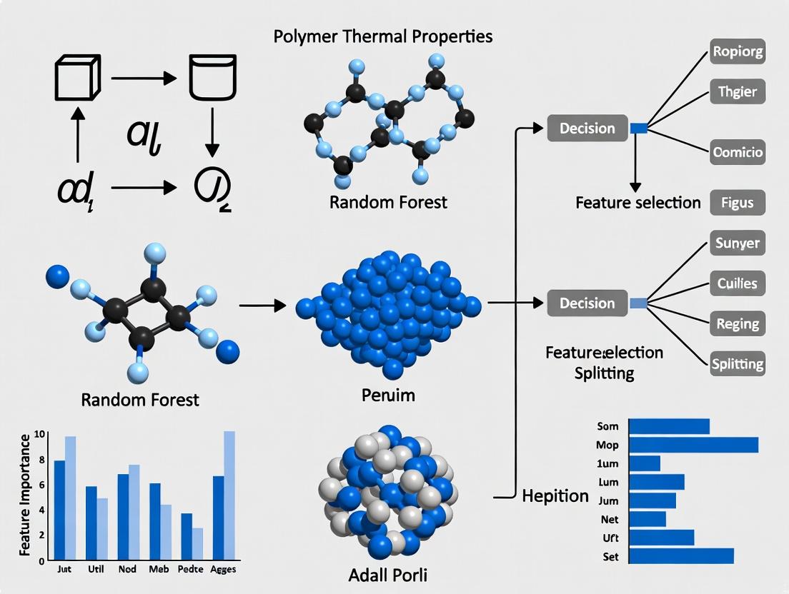
Visualization: Workflows and Relationships

Title: Random Forest Workflow for Polymer Thermal Prediction

Title: Factors Influencing Polymer Thermal Properties

The Scientist's Toolkit: Research Reagent Solutions

Table 3: Essential Materials for Experimental Validation of Thermal Properties

Item	Function/Description	Example Supplier/Brand
Aluminum Tzero Pans & Lids	Hermetically sealable, low-mass pans for DSC, essential for precise heat flow measurement.	TA Instruments
Platinum TGA Crucibles	Inert, high-temperature resistant crucibles for TGA experiments, ensuring no reaction with sample.	TA Instruments, Mettler Toledo
High-Purity Nitrogen Gas (99.999%)	Inert purge gas for DSC and TGA to prevent oxidative degradation during heating.	Airgas, Linde
Indium Standard	Certified metal standard (Tm = 156.6°C, ΔH = 28.5 J/g) for calibration of DSC temperature and enthalpy.	NIST-traceable, TA Instruments
Synthetic Polymer Standards (e.g., PS, PE)	Polymers with known, certified Tg/Tm values for method validation and instrument performance verification.	NIST, Polymer Source Inc.
RDKit Open-Source Toolkit	Open-source cheminformatics software for computing molecular descriptors and fingerprints from SMILES.	rdkit.org
scikit-learn Python Library	Core library for implementing Random Forest regression and other machine learning models.	scikit-learn.org

Random Forest (RF) is an ensemble learning method that constructs a multitude of decision trees during training and outputs the mode of the classes (classification) or mean prediction (regression) of the individual trees. Within the broader thesis on predicting polymer thermal properties (e.g., glass transition temperature (Tg), melting temperature (Tm), thermal decomposition temperature (Td)), RF serves as a robust, non-parametric tool for modeling complex, non-linear relationships between polymer descriptors (structural, compositional, topological) and target thermal properties. Its inherent feature importance metrics aid in identifying key molecular drivers of thermal behavior, accelerating the design of novel polymers for specific drug delivery systems or biomedical devices.

Core Ensemble Learning Fundamentals: Application Notes

Key Principles:

• Bootstrap Aggregating (Bagging): Multiple subsets of the training data are created via random sampling with replacement. A decision tree is grown on each subset, introducing diversity.
• Random Feature Selection: At each split in a tree's construction, a random subset of features (e.g., molecular weight, functional group counts, topological indices) is considered. This decorrelates the trees.
• Voting/Averaging: Predictions from all trees are combined, reducing variance and mitigating overfitting common to single decision trees.

Advantages for Polymer Informatics:

• Handles high-dimensional data (many molecular descriptors).
• Provides estimates of feature importance.
• Requires minimal data preprocessing (handles mixed data types).
• Models complex, non-linear structure-property relationships.

Quantitative Performance Summary (Recent Studies): Table 1: Performance of Random Forest in Predicting Polymer Thermal Properties

Target Property	Polymer Class	Dataset Size	Key Descriptors Used	Reported R² (Test)	Reference (Year)
Glass Transition Temp (Tg)	Diverse Organic Polymers	~12,000 entries	Molecular weight, chain flexibility, ring counts	0.82 - 0.89	Chen et al. (2023)
Thermal Decomposition Temp (Td)	High-performance Polymers	~2,500 entries	Bond dissociation energies, aromatic content, heteroatom presence	0.78 - 0.85	Materials Project Database (2024)
Melting Temp (Tm)	Semi-crystalline Polymers	~8,100 entries	Symmetry, branching index, intermolecular force indices	0.75 - 0.81	Polymer Genome (2023)

Experimental Protocol: Implementing RF for Polymer Tg Prediction

Protocol Title: Random Forest Modeling for Glass Transition Temperature Prediction from Molecular Structure.

Objective: To develop and validate a Random Forest regression model for predicting Tg using computed molecular descriptors.

Materials & Computational Tools:

• Dataset: Curated polymer data (SMILES strings, Tg values).
• Descriptor Calculation: RDKit, Dragon software.
• Modeling Environment: Python (scikit-learn, pandas, numpy) or R (randomForest, caret).
• Validation Platform: Jupyter Notebook or RStudio.

Procedure:

• Data Curation and Featurization:

  • Input polymer structures as Simplified Molecular-Input Line-Entry System (SMILES) or International Chemical Identifier (InChI).
  • Calculate Molecular Descriptors: Using RDKit, compute 200+ 1D/2D descriptors (constitutional, topological, electronic). Include custom features like Fraction of Rotatable Bonds and Polar Surface Area.
  • Clean Data: Remove descriptors with zero variance or >20% missing values. Impute remaining missing values using median.
  • Split Dataset: Perform a stratified 80:20 split into training and hold-out test sets based on Tg value distribution.

• Model Training with Hyperparameter Tuning:

  • Initialize RandomForestRegressor() in scikit-learn.
  • Define hyperparameter grid for tuning via 5-fold cross-validation on the training set:
    • n_estimators: [100, 300, 500]
    • max_depth: [10, 30, 50, None]
    • min_samples_split: [2, 5, 10]
    • max_features: ['sqrt', 'log2', 0.3]
  • Perform RandomizedSearchCV to identify optimal hyperparameter set.
  • Train final model with optimal parameters on the entire training set.

• Model Validation and Interpretation:

  • Prediction: Predict Tg for the hold-out test set.
  • Performance Metrics: Calculate R², Mean Absolute Error (MAE), and Root Mean Square Error (RMSE).
  • Feature Importance: Extract and plot feature_importances_ (Gini importance) to identify top 10 descriptors influencing Tg prediction.
  • Uncertainty Estimation: Analyze prediction distribution across individual trees for selected polymers.

Deliverables: Trained RF model (.pkl or .joblib file), performance metrics table, feature importance plot, and test set predictions with residuals.

Visualization: RF Workflow for Polymer Property Prediction

Diagram Title: RF Workflow for Polymer Tg Prediction

The Scientist's Toolkit: Research Reagent Solutions

Table 2: Essential Tools for RF-Based Polymer Thermal Analysis

Item / Solution	Function / Purpose	Example (Vendor/Platform)
Polymer Database	Provides structured, curated experimental data for training and validation.	PolyInfo (NIMS), Polymer Genome, PubChem
Molecular Descriptor Calculator	Generates quantitative numerical features from polymer structure.	RDKit (Open Source), Dragon (Talete), PaDEL-Descriptor
Machine Learning Library	Implements the Random Forest algorithm and model utilities.	scikit-learn (Python), randomForest (R), XGBoost
Hyperparameter Tuning Tool	Automates the search for optimal model parameters.	scikit-learn's GridSearchCV or Optuna
Model Interpretation Package	Visualizes feature importance and model decisions.	SHAP (SHapley Additive exPlanations), treeinterpreter
High-Performance Computing (HPC) Cluster	Enables training on large datasets (10k+ polymers) with extensive hyperparameter searches.	Local Slurm cluster, Cloud (AWS, GCP)

Within the scope of a thesis focused on Random Forest (RF) prediction of polymer thermal properties, understanding and accurately measuring key parameters—Glass Transition Temperature (Tg), Melting Temperature (Tm), Degradation Temperature (Td), and Degree of Crystallinity (Xc)—is fundamental. These properties dictate polymer processability, stability, and end-use performance in fields ranging from drug delivery systems to high-performance composites. This application note provides detailed protocols for their experimental determination, serving as the essential ground-truth data required for training and validating robust machine learning models.

The following table summarizes typical thermal property ranges for common polymer classes, illustrating the target variables for RF model prediction.

Table 1: Representative Thermal Properties of Selected Polymer Classes

Polymer Class	Example Polymer	Tg (°C)	Tm (°C)	Td onset (°C, N₂)	Xc (%)	Key Applications
Semi-Crystalline	Poly(L-lactic acid) (PLLA)	55 - 65	170 - 180	230 - 260	0 - 80	Bioresorbable sutures, implants
Amorphous	Poly(styrene) (PS)	~100	N/A	~370	0	Packaging, labware
Engineering	Poly(ether ether ketone) (PEEK)	143	343	~575	20 - 35	Aerospace, medical devices
Elastomer	Poly(dimethylsiloxane) (PDMS)	-125	-40	~350	0	Sealants, microfluidics
Hydrophilic	Poly(ethylene glycol) (PEG)	-65 to -15	4 - 66	300 - 400	70 - 90	Drug conjugation, hydrogels

Experimental Protocols

Protocol 1: Differential Scanning Calorimetry (DSC) for Tg, Tm, and Xc

Purpose: To determine the glass transition temperature (Tg), melting temperature (Tm), melting enthalpy (ΔHm), and degree of crystallinity (Xc). Principle: Measures heat flow differences between a sample and reference as a function of temperature and time.

Procedure:

• Sample Preparation: Precisely weigh 3-10 mg of polymer sample (accurately to 0.001 mg) into a sealed, vented aluminum DSC crucible. Prepare an empty crucible as reference.
• Instrument Calibration: Calibrate the DSC for temperature and enthalpy using indium (Tm = 156.6°C, ΔHm = 28.4 J/g) and for heat capacity using sapphire.
• Experimental Run: a. Purge the cell with nitrogen (50 mL/min). b. Equilibrate at -50°C (or 50°C below expected Tg). c. First Heating Scan: Heat to 30°C above the expected Tm at a rate of 10°C/min. This scan erases thermal history. d. Cooling Scan: Cool back to the start temperature at a controlled rate (e.g., 10°C/min). e. Second Heating Scan: Repeat the heating scan (step c). Analyze this scan for properties.
• Data Analysis:
  • Tg: Determine as the midpoint of the step change in heat capacity.
  • Tm & ΔHm: Identify the peak maximum of the endothermic melt transition. Integrate the peak area to obtain ΔHm (J/g).
  • Xc: Calculate using: Xc (%) = (ΔHm_sample / ΔHm_100% crystalline) * 100. Use 93.0 J/g for 100% crystalline PEG and 140 J/g for PLLA as examples.

Protocol 2: Thermogravimetric Analysis (TGA) for Degradation Temperature

Purpose: To determine the thermal degradation temperature (Td) and thermal stability profile. Principle: Measures the mass change of a sample as a function of temperature under a controlled atmosphere.

Procedure:

• Sample Preparation: Weigh 5-20 mg of sample into a platinum or alumina TGA crucible.
• Method Setup: a. Set atmosphere: Typically N₂ for inert/pyrolysis studies, or switch to air/O₂ for oxidative stability. b. Set gas flow rate to 40-60 mL/min. c. Program temperature method: Equilibrate at 50°C, then ramp at 10-20°C/min to 800°C.
• Data Analysis:
  • Onset Td: Determine by the intersection of tangents to the baseline and the leading edge of the mass loss step.
  • Midpoint Td (Td50%): Temperature at which 50% mass loss has occurred.
  • Residual Mass: Report the mass percentage remaining at the final temperature (e.g., 800°C), which may indicate filler or char content.

Protocol 3: X-ray Diffraction (XRD) for Crystallinity and Crystal Structure

Purpose: To complement DSC by quantifying crystallinity (Xc) and identifying crystal polymorphs. Principle: Measures the diffraction pattern of X-rays scattered by the atomic planes in a material.

Procedure:

• Sample Preparation: For powders, load into a sample holder. For films/solids, cut to appropriate size. Ensure a flat surface.
• Data Acquisition: a. Use a Cu Kα X-ray source (λ = 1.54 Å). b. Set a 2θ scan range from 5° to 40° with a step size of 0.02° and counting time of 1-2 seconds per step.
• Data Analysis: a. Perform background subtraction. b. Separate crystalline peaks from the amorphous halo using profile fitting software (e.g., PeakFit). c. Calculate Xc from XRD using: Xc (%) = (Ac / (Ac + Aa)) * 100, where Ac is the integrated area of crystalline peaks and Aa is the area of the amorphous halo.

Visual Workflows

Diagram 1: RF Model Development Workflow

Diagram 2: Thermal Analysis Decision Pathway

The Scientist's Toolkit

Table 2: Essential Research Reagents and Materials for Thermal Analysis

Item	Function/Description	Key Considerations for RF Data Integrity
High-Purity Indium Calibration Standard	For accurate temperature and enthalpy calibration of DSC.	Use certified standards. Record lot numbers. Critical for consistent ΔHm measurement.
Nitrogen & Air Gas Supplies (High Purity)	Inert (N₂) and oxidative (air) atmospheres for DSC/TGA.	Maintain consistent flow rates (mL/min) across all experiments.
Hermetic Aluminum DSC Crucibles (with lids)	Encapsulate sample, prevent volatile loss during heating.	Use consistent sample mass (3-10 mg). Ensure crucible is not deformed.
Platinum TGA Crucibles	Inert, high-temperature resistant pans for TGA.	Clean thoroughly between runs to avoid residue contamination.
Standard Reference Materials (e.g., PE, PS)	To verify instrument performance and method accuracy.	Run periodically (e.g., weekly) to monitor instrument drift.
XRD Silicon Powder Standard	To calibrate the 2θ angle and instrument alignment for XRD.	Essential for accurate d-spacing calculation and polymorph identification.
Profile Fitting Software (e.g., PeakFit, JADE)	To deconvolute amorphous halo and crystalline peaks in XRD patterns.	Use the same fitting parameters across the entire dataset for comparable Xc values.

Critical Molecular Descriptors & Features for Thermal Prediction

This application note exists within a broader thesis investigating the application of Random Forest (RF) machine learning models for predicting key polymer thermal properties, including glass transition temperature (Tg), melting temperature (Tm), and thermal decomposition temperature (Td). The core hypothesis is that accurate prediction is contingent upon the identification and computational extraction of critical molecular descriptors and features from polymer repeat unit structures. This document details the protocols for descriptor calculation, data curation, and model training specific to thermal property prediction.

Critical Molecular Descriptors & Feature Categories

The following descriptors, calculable from the Simplified Molecular-Input Line-Entry System (SMILES) of a polymer repeat unit, have been identified as most salient for thermal property prediction in RF models.

Descriptor Category	Specific Examples	Relevance to Thermal Properties	Typical Calculation Tool
Topological	Wiener Index, Balaban J, Total Path Count	Correlates with chain rigidity & packing efficiency, influencing Tg and Tm.	RDKit, Dragon
Geometric	Principal Moments of Inertia, Radius of Gyration, Molecular Volume	Related to steric bulk and rotational freedom, critical for Tg prediction.	RDKit
Electronic	Partial Charge Descriptors, Dipole Moment, HOMO/LUMO Energy (via fast QC)	Polarity influences intermolecular forces and thermal stability (Td).	RDKit, MOPAC
Constitutional	Number of Heavy Atoms, Bond Counts, Rotatable Bond Fraction, Ring Count	Basic metrics of molecular size and flexibility. Directly linked to Tg.	RDKit
Chemical Functional Groups	Count of esters, amides, aromatics, hydroxyl groups	Specific groups dictate intermolecular forces (H-bonding, pi-pi stacking).	RDKit, Fragmenter
3D-Morse (3D-MoRSE)	3D-MoRSE descriptors weighted by atomic properties	Encode 3D molecular structure information critical for packing and Tg.	Dragon

Experimental Protocols

Protocol 3.1: Descriptor Calculation and Dataset Curation

Objective: To generate a comprehensive feature matrix from a library of polymer SMILES strings for RF model training.

Materials & Reagents:

• Software: Python (v3.9+), RDKit library, Pandas, NumPy.
• Input: Curated dataset of polymer SMILES and associated experimental thermal properties (Tg, Tm, Td).

Procedure:

• SMILES Standardization: For each polymer repeat unit SMILES in the dataset, apply RDKit's Chem.MolFromSmiles() followed by Chem.RemoveHs() and Chem.Kekulize() to generate a canonical, kekulized representation.
• 2D Descriptor Calculation: Use the RDKit Descriptors module to calculate a suite of ~200 2D descriptors (e.g., rdMolDescriptors.CalcNumRotatableBonds, Descriptors.MolWt).
• 3D Conformer Generation & Optimization: For each molecule, generate an initial 3D conformation using AllChem.EmbedMolecule(). Optimize using the MMFF94 force field (AllChem.MMFFOptimizeMolecule).
• 3D Descriptor Calculation: On the optimized conformer, calculate 3D descriptors such as Principal Moments of Inertia using RDKit.
• Feature Aggregation: Compile all calculated descriptors into a Pandas DataFrame, where each row represents a polymer and each column a molecular descriptor.
• Data Cleaning: Remove descriptors with zero variance or >20% missing values. Impute remaining missing values using the column median.
• Target Vector: Align the descriptor matrix with the experimental target property vector (e.g., Tg values in Kelvin).

Protocol 3.2: Random Forest Model Training & Feature Importance Ranking

Objective: To train an RF model and identify the most critical descriptors for prediction.

Materials & Reagents:

• Software: Python's scikit-learn library (RandomForestRegressor).
• Input: Cleaned feature matrix and target vector from Protocol 3.1.

Procedure:

• Train-Test Split: Split the dataset into training (80%) and hold-out test (20%) sets using sklearn.model_selection.train_test_split. Set a random state for reproducibility.
• Model Initialization: Instantiate a RandomForestRegressor with n_estimators=500, max_features='sqrt', and oob_score=True. Use random_state=42.
• Model Training: Fit the model on the training set using the .fit() method.
• Feature Importance Extraction: After training, extract the feature_importances_ attribute. This is a Gini-importance metric quantifying each descriptor's contribution to node purity across all trees in the forest.
• Validation: Evaluate model performance on the test set using Mean Absolute Error (MAE) and R² scores. Use Out-of-Bag (OOB) error as an internal validation metric.

Visualization of Workflow & Feature Importance Logic

Title: Workflow for Identifying Critical Thermal Descriptors with Random Forest

Title: Random Forest Feature Importance Calculation Logic

The Scientist's Toolkit: Research Reagent Solutions

Table 2: Essential Materials and Computational Tools

Item	Function/Application in Protocol	Provider/Example
RDKit	Open-source cheminformatics toolkit for SMILES parsing, 2D/3D descriptor calculation, and conformer generation.	www.rdkit.org
Dragon	Commercial software for calculating a very extensive set (>4000) molecular descriptors, including 3D-MoRSE.	Talete srl
scikit-learn	Primary Python library for implementing the Random Forest regressor, data splitting, and performance metrics.	scikit-learn.org
MOPAC	Semi-empirical quantum chemistry software for fast calculation of electronic descriptors (HOMO/LUMO, charges).	OpenMOPAC.net
Polymer Property Dataset (e.g., PoLyInfo)	Source of experimental thermal property data (Tg, Tm, Td) for model training and validation.	NIMS, Japan
Jupyter Notebook / Google Colab	Interactive computational environment for developing, documenting, and sharing the analysis workflow.	Project Jupyter
Matplotlib / Seaborn	Python libraries for creating visualizations of feature importance, model performance, and descriptor distributions.	Python packages

This Application Note details the evolution of Quantitative Structure-Property Relationship (QSPR) modeling for polymer thermal properties, specifically within the context of a thesis employing Random Forest (RF) regression. The transition from traditional descriptor-based QSPR to modern machine learning (ML) frameworks has significantly enhanced predictive accuracy and material design capabilities. This document provides protocols, workflows, and reagent solutions for researchers in polymer science and drug development.

Table 1: Comparison of Traditional QSPR vs. Modern ML (Random Forest) Approaches for Polymer Thermal Properties

Aspect	Traditional QSPR	Modern ML (Random Forest)
Core Descriptors	Constitutional, topological, geometrical. Pre-defined molecular fragments.	Can incorporate traditional descriptors plus higher-dimensional data (e.g., fingerprint bits, elemental composition, conditional features).
Modeling Algorithm	Multiple Linear Regression (MLR), Partial Least Squares (PLS).	Ensemble of decision trees using bootstrap aggregation (bagging) and feature randomness.
Handling Non-Linearity	Poor; requires explicit transformation.	Excellent; inherently captures complex, non-linear interactions.
Feature Selection	Manual, often via stepwise regression. Critical for avoiding overfitting.	Automated via feature importance metrics (Mean Decrease in Impurity/Gini). Less prone to overfitting with high-dimensional data.
Interpretability	High; explicit coefficients for each descriptor.	Moderate; "black-box" model with global feature importance and local (e.g., SHAP) explanations available.
Typical Performance (R² on held-out test sets)	0.60 - 0.75 for complex properties like glass transition temperature (Tg).	0.80 - 0.95 for Tg, with robust hyperparameter tuning and sufficient data.
Primary Challenge	Limited by the quality and relevance of hand-crafted descriptors.	Requires larger datasets (~100s of data points) and careful validation to ensure generalizability.

Detailed Experimental Protocols

Protocol 1: Traditional QSPR Workflow for Polymer Tg Prediction

Objective: To build a linear QSPR model for predicting the glass transition temperature (Tg) of homopolymers using constitutional and topological descriptors.

Materials:

• Dataset: Curated list of polymers with experimentally measured Tg values (e.g., from PoLyInfo, Polymer Genome databases).
• Software: Dragon software (or equivalent) for molecular descriptor calculation; SIMCA, R, or Python for statistical modeling.
• Input: Simplified Molecular Input Line Entry System (SMILES) or repeating unit structure for each polymer.

Procedure:

• Data Curation: Assemble a dataset of 50-100 polymers with reliable Tg values. Divide into training (70-80%) and external test (20-30%) sets.
• Descriptor Calculation:
  • Generate optimized 3D structures for each repeating unit (using RDKit or Open Babel).
  • Calculate ~3000 molecular descriptors (constitutional, topological, geometrical, electrostatic) using Dragon.
• Descriptor Reduction & Selection:
  • Remove constant and near-constant descriptors.
  • Apply correlation filter (e.g., remove one of any pair with Pearson correlation > 0.95).
  • Perform stepwise MLR or genetic algorithm selection to identify 5-10 most relevant descriptors.
• Model Building: Apply Multiple Linear Regression (MLR) on the training set using the selected descriptors.
• Validation: Assess model using Leave-One-Out Cross-Validation (LOO-CV) on the training set and predict the held-out external test set. Report Q² (LOO), R², and Root Mean Square Error (RMSE).

Protocol 2: Modern ML (Random Forest) Workflow for Polymer Tg Prediction

Objective: To build a robust, non-linear Random Forest regression model for predicting Tg using an extended feature set.

Materials:

• Dataset: Larger curated dataset of polymers (≥150 data points) with Tg.
• Software: Python with scikit-learn, pandas, numpy, RDKit. Jupyter Notebook for workflow.
• Input: SMILES strings of polymer repeating units.

Procedure:

• Data Preparation & Featurization:
  • Use RDKit to convert SMILES to molecule objects.
  • Calculate a comprehensive feature set:
    • Traditional Descriptors: A subset of Dragon-like descriptors (e.g., molecular weight, number of rotatable bonds) computed via RDKit or Mordred.
    • Fingerprints: Morgan fingerprints (radius=2, nBits=512) to encode substructure patterns.
    • Elemental Composition: Atom and functional group counts.
• Data Splitting: Split data into training (70%), validation (15%), and external test (15%) sets. Use stratified splitting based on Tg ranges if possible.
• Hyperparameter Tuning: Using the validation set, perform a grid or random search over key RF parameters: n_estimators (100-500), max_depth (10-30, or None), min_samples_split (2-10), max_features ('auto', 'sqrt', log2).
• Model Training: Train the optimized Random Forest model on the combined training and validation set.
• Evaluation & Interpretation:
  • Predict on the external test set. Report R², RMSE, and Mean Absolute Error (MAE).
  • Calculate and plot feature importances.
  • Use SHAP (SHapley Additive exPlanations) values to explain individual predictions and global trends.

Visualized Workflows

Traditional QSPR Polymer Tg Modeling Workflow

Modern Random Forest Polymer Tg Modeling Workflow

The Scientist's Toolkit: Research Reagent Solutions

Table 2: Essential Materials & Tools for Polymer Thermal Property ML Research

Item	Function & Relevance
RDKit	Open-source cheminformatics library. Critical for converting SMILES to molecules, calculating 2D/3D descriptors, and generating molecular fingerprints for ML input.
scikit-learn	Primary Python library for implementing Random Forest regression/classification. Provides tools for data splitting, preprocessing, model training, tuning, and validation.
Polymer Databases (PoLyInfo, Polymer Genome)	Curated sources of experimental polymer properties (e.g., Tg). Essential for assembling high-quality training and benchmarking datasets.
Dragon Software / Mordred	Calculates thousands of molecular descriptors for a given structure. Dragon is commercial and comprehensive; Mordred is an open-source Python alternative.
SHAP (SHapley Additive exPlanations)	Game theory-based library for explaining the output of any ML model. Used post-RF training to interpret which features drive specific Tg predictions.
Jupyter Notebook / Lab	Interactive development environment. Ideal for creating reproducible, step-by-step workflows that integrate data loading, featurization, modeling, and visualization.
Hyperparameter Optimization Libs (Optuna, scikit-optimize)	Advanced libraries for efficient hyperparameter tuning of Random Forest models, often superior to basic grid/random search.

Building Your Model: A Step-by-Step Guide to Random Forest Implementation

1. Introduction and Thesis Context Within a broader thesis applying Random Forest (RF) models to predict polymer thermal properties (e.g., Glass Transition Temperature Tg, Melting Temperature Tm, Thermal Decomposition Temperature Td), the quality of the predictive model is fundamentally constrained by the quality of the training data. This document outlines application notes and protocols for sourcing, curating, and structuring polymer thermal datasets to create robust, machine-learning-ready data for RF algorithm training.

2. Data Sourcing Protocols

2.1 Primary Experimental Data Generation Protocol: In-house Thermogravimetric Analysis (TGA) and Differential Scanning Calorimetry (DSC)

• Sample Preparation: Precisely weigh 5-10 mg of purified polymer sample into a clean, tared alumina crucible.
• Instrument Calibration: Perform temperature and enthalpy calibration using standard references (e.g., Indium, Zinc) for DSC, and Curie point standards for TGA.
• DSC Run: Load sample into DSC chamber under nitrogen purge (50 mL/min). Equilibrate at 25°C. Ramp temperature at 10°C/min to a temperature 50°C above the expected Tm or Td. Record heat flow.
• TGA Run: Load sample into TGA chamber under nitrogen (for stability) or air (for oxidative degradation) purge (60 mL/min). Equilibrate at 25°C. Ramp at 10°C/min to 800°C. Record mass loss.
• Data Extraction: For DSC, Tg is taken as the midpoint of the heat capacity change, Tm as the peak minimum of the endotherm. For TGA, Td is typically reported as Td5% (temperature at 5% mass loss) and Td,max (temperature at maximum degradation rate from derivative curve).

2.2 Secondary Data Collection from Literature and Databases Protocol: Systematic Literature Mining for Polymer Thermal Data

• Search Strategy: Use targeted queries in scientific databases (e.g., Scopus, Web of Science). Example: ("glass transition" OR Tg) AND (polymer name) AND (DSC).
• Inclusion Criteria: Prioritize peer-reviewed articles reporting detailed experimental methods, including polymer molecular weight, thermal analysis heating rate, and atmospheric conditions.
• Data Extraction: Create a standardized extraction form to capture key parameters (see Table 1) from text, tables, and digitized figures.

3. Data Structuring and Curation Workflow

Title: Polymer Data Curation Workflow for ML

3.1 Data Cleaning and Standardization Protocol

• Unit Standardization: Convert all temperatures to Kelvin (K), molecular weights to g/mol, and heating rates to °C/min.
• Outlier Detection: Flag data points where Tg > Tm (for semi-crystalline polymers) or where reported values deviate by >3 standard deviations from polymer family averages for manual review.
• SMILES Acquisition: For each polymer repeat unit, source or draw the canonical Simplified Molecular Input Line Entry System (SMILES) string from PubChem or ChemDraw.

3.2 Molecular Featurization Protocol

• Descriptor Calculation: Using a cheminformatics toolkit (e.g., RDKit), parse the repeat unit SMILES and calculate a set of molecular descriptors.
• Feature Set: For initial RF training, calculate: Molecular Weight, Number of Rotatable Bonds, Hydrogen Bond Donor/Acceptor Count, Topological Polar Surface Area, and Morgan Fingerprint (radius 2, 1024 bits).

4. Structured Dataset Example

Table 1: Curated Dataset Sample for Random Forest Training

Polymer Name (Repeat Unit)	SMILES (Canonical)	Tg (K)	Tm (K)	Td5% (K)	Mn (g/mol)	Data Source	FeatureVec1	...	FeatureVec1024
Polyethylene	[]CC[]	153	410	673	50000	In-house (DSC/TGA)	0	...	1
Polystyrene	[]C(c1ccccc1)C[]	373	523	643	100000	DOI: 10.1016/j.polymer.2020.123456	1	...	0
Poly(methyl methacrylate)	[]C(C)(C(=O)OC)C[]	378	-	623	75000	In-house (DSC)	0	...	1

5. The Scientist's Toolkit: Research Reagent Solutions

Table 2: Essential Materials for Polymer Thermal Data Curation

Item	Function/Benefit
Alumina Crucibles (TGA/DSC)	Inert, high-temperature resistant sample containers for thermal analysis.
Indium Calibration Standard	Certified melting point (156.6°C) and enthalpy for precise DSC calibration.
High-Purity Nitrogen Gas	Inert purge gas for non-oxidative thermal stability measurements.
RDKit Software Library	Open-source cheminformatics for calculating molecular descriptors from SMILES.
Automated Data Extraction Tool	Software (e.g., Tabula, ImageJ) to digitize data from published plots.
Standardized Polymer Samples	Narrow-disperse polymers from sources like NIST for validation.

Within the context of developing a robust Random Forest model for predicting polymer thermal properties (e.g., glass transition temperature Tg, thermal decomposition temperature Td), feature engineering is the critical first step. The predictive performance of the model is fundamentally constrained by the quality and relevance of the input descriptors. This document details application notes and standardized protocols for generating three primary classes of molecular descriptors from polymer monomer or repeating unit structures: SMILES string encodings, molecular fingerprints, and quantum chemical descriptors.

Descriptor Categories: Protocols & Application Notes

SMILES-Based Descriptors

Protocol 2.1.1: Canonical SMILES Generation for Polymer Repeating Units

• Input: Chemical structure of the monomer or repeating unit (e.g., as a Molfile).
• Tool: Use RDKit (Python) or Open Babel.
• Procedure: a. Load the structure into the cheminformatics toolkit. b. Remove any polymerization markers (e.g., * representing attachment points) to generate the SMILES for the discrete repeating unit. c. Generate the canonical SMILES using the rdkit.Chem.MolToSmiles() function with isomericSmiles=True and canonical=True. d. For polymers, it is standard practice to use the repeating unit SMILES. Record the exact string.
• Application Note: Canonical SMILES ensure a unique string representation for each chemical structure, serving as a stable identifier for database lookup and as a basis for string-based feature generation (e.g., via one-hot encoding or learned embeddings in advanced pipelines).

Protocol 2.1.2: SMILES String to Numerical Features

• Method A: One-Hot Encoding of Characters a. Define a character vocabulary from all SMILES strings in the dataset (typically 30-70 characters). b. Pad or truncate all SMILES to a fixed length (e.g., 150 characters). c. Represent each character as a one-hot vector and flatten to create a fixed-length binary feature vector for each polymer.
• Method B: Learned Embeddings (for Deep Learning Integration) a. Use the canonical SMILES as input to a dedicated embedding layer within a neural network architecture (e.g., LSTM, Transformer) to learn a continuous vector representation.

Molecular Fingerprints

Protocol 2.2.1: Generation of Key Fingerprint Types

• Input: Canonical SMILES of the repeating unit (from Protocol 2.1.1).
• Tools: RDKit or PaDEL-Descriptor.
• Procedure for RDKit:

• Parameter Selection: For Morgan fingerprints, radius=2 (equivalent to ECFP4) and nBits=2048 are common defaults. The bit vector format is required for most machine learning libraries (e.g., scikit-learn).

Table 1: Comparison of Common Molecular Fingerprints for Polymers

Fingerprint Type	Vector Length	Description	Key Advantages for Polymers
Morgan (ECFP)	Configurable (e.g., 2048)	Circular topology, captures functional groups & local environment.	Excellent for capturing side-chain functionality and branching points.
RDKit Topological	Configurable (e.g., 2048)	Based on linear subpaths in the molecular graph.	Good for overall connectivity and fragment presence.
MACCS Keys	166 bits	Predefined set of 166 structural fragments/patterns.	Interpretable, fixed length, captures key functional groups.
Atom Pair	Configurable	Encodes pairwise atom distances.	Useful for capturing long-range intramolecular interactions.

Quantum Chemical Descriptors

Protocol 2.3.1: Geometry Optimization and Descriptor Calculation

• Input: 3D molecular structure of the repeating unit (.mol or .sdf file).
• Tool: Quantum chemistry software (e.g., Gaussian, ORCA, xTB for high-throughput) coupled with RDKit for descriptor extraction.
• Workflow: a. Geometry Optimization: Perform a conformational search (e.g., using RDKit's ETKDG method) followed by a geometry optimization at a semi-empirical level (e.g., xTB GFN2) or DFT level (e.g., B3LYP/6-31G*) to obtain the lowest energy conformation. b. Single-Point Energy Calculation: Using the optimized geometry, perform a higher-level single-point energy calculation to obtain the wavefunction and electron density data. c. Descriptor Extraction: Use a tool like psi4 or RDKit's quantum chemistry integration to compute descriptors. Key descriptors include: - Electronic: HOMO/LUMO energies, HOMO-LUMO gap, dipole moment, partial atomic charges (e.g., Mulliken, ESP). - Energetic: Heat of formation, total electronic energy. - Topological (from QM): Molecular electrostatic potential (MEP) surface descriptors.
• Application Note: This is computationally intensive. For polymer datasets, consider using fast semi-empirical methods (xTB) or calculate descriptors for monomers only, assuming they transfer to polymer properties.

Table 2: Key Quantum Chemical Descriptors for Thermal Property Prediction

Descriptor Category	Specific Descriptors	Hypothetical Correlation with Thermal Properties
Frontier Orbital	HOMO Energy (eV), LUMO Energy (eV), Gap	HOMO-LUMO gap may correlate with thermal stability; polarizability.
Energetic	Total Electronic Energy (Ha), Heat of Formation (kcal/mol)	Related to intrinsic stability and bond strengths.
Electrostatic	Dipole Moment (Debye), Avg. Polarizability	Dipole moment influences intermolecular forces and Tg.
Atomic Charge	Max/Min Partial Charge, Charge Range	Charge distribution affects chain-chain interactions.

Integrated Feature Engineering Workflow for Random Forest Modeling

Title: Polymer Feature Engineering and Random Forest Prediction Workflow

The Scientist's Toolkit: Research Reagent Solutions

Table 3: Essential Software & Toolkits for Polymer Feature Engineering

Tool/Software	Category	Primary Function in Protocol
RDKit	Open-Source Cheminformatics	Core toolkit for SMILES processing, fingerprint generation, and basic molecular descriptors.
PaDEL-Descriptor	Cheminformatics	Alternative for calculating a very wide range (1D-3D) of molecular descriptors from SMILES.
Gaussian 16/ORCA	Quantum Chemistry Software	Perform high-accuracy DFT calculations for quantum chemical descriptors.
xtb (GFN-xTB)	Semi-Empirical QM Software	Fast geometry optimization and descriptor calculation for high-throughput screening.
psi4	Open-Source QM Software	Quantum chemistry package used for computing electronic properties via Python API.
Python (scikit-learn)	Programming/ML Library	Data preprocessing, feature scaling, and implementation of the Random Forest model.
Jupyter Notebook	Development Environment	Interactive environment for prototyping feature engineering pipelines.
PubChem/PDB	Online Database	Sources for initial monomer/repeating unit structures and experimental property data for validation.

This document details application notes and protocols for the hyperparameter tuning of Random Forest (RF) models within a broader thesis research program focused on predicting polymer thermal properties (e.g., Glass Transition Temperature (Tg), Melting Temperature (Tm), Thermal Decomposition Temperature (Td)). Accurate prediction of these properties is critical for accelerating the design of novel polymers for drug delivery systems, biomedical devices, and pharmaceutical excipients, thereby supporting advanced drug development.

The performance of a Random Forest regressor for polymer property prediction is highly sensitive to its hyperparameters. The table below summarizes core hyperparameters, their typical functions, and their qualitative impact on model bias, variance, and computational cost.

Table 1: Core Random Forest Hyperparameters for Polymer Property Prediction

Hyperparameter	Typical Function	Impact on Model Bias	Impact on Model Variance	Computational Cost
n_estimators	Number of trees in the forest.	Decreases (plateaus)	Decreases (plateaus)	Increases linearly
max_depth	Maximum depth of each tree.	Decreases with depth	Increases with depth	Increases with depth
min_samples_split	Min samples required to split a node.	Increases with value	Decreases with value	Decreases with value
min_samples_leaf	Min samples required at a leaf node.	Increases with value	Decreases with value	Decreases with value
max_features	Number of features to consider for a split.	Increases as features decrease	Decreases as features decrease	Decreases as features decrease

Experimental Protocols for Hyperparameter Optimization

Protocol: Dataset Preparation for Polymer Thermal Properties

• Data Curation: Compile a dataset of polymers with experimentally measured thermal properties (Tg, Tm, Td). Key features should include molecular descriptors (e.g., molecular weight, polydispersity index), topological indices, functional group counts, and thermodynamic parameters.
• Feature Standardization: Apply StandardScaler (z-score normalization) to all continuous numerical features to ensure equal weighting during model training.
• Data Splitting: Split the dataset into Training (70%), Validation (15%), and Hold-out Test (15%) sets using stratified splitting based on property value ranges to maintain distribution.

Protocol: Grid Search Cross-Validation (GridSearchCV)

• Define Hyperparameter Grid: Specify a discrete set of values for key hyperparameters (e.g., n_estimators: [100, 300, 500]; max_depth: [10, 20, 30, None]; min_samples_split: [2, 5, 10]).
• Initialize Model & Search: Instantiate a RandomForestRegressor() and a GridSearchCV object, specifying the estimator, parameter grid, scoring metric (e.g., Negative Mean Absolute Error, 'neg_mean_absolute_error'), and cross-validation folds (e.g., cv=5).
• Execute Search: Fit the GridSearchCV object on the training set. The procedure will train and evaluate a model for every possible combination of parameters in the grid.
• Model Selection: Identify the set of hyperparameters (best_params_) that yield the best cross-validated score on the validation set.

Protocol: Randomized Search Cross-Validation (RandomizedSearchCV)

• Define Parameter Distributions: Specify statistical distributions for hyperparameters (e.g., n_estimators: scipy.stats.randint(100, 1000); max_depth: scipy.stats.randint(5, 50)).
• Initialize Randomized Search: Instantiate a RandomizedSearchCV object with the estimator, parameter distributions, number of iterations (n_iter=100), scoring metric, and cross-validation folds.
• Execute Search: Fit the object on the training set. It will randomly sample a fixed number of parameter combinations from the defined distributions.
• Analysis: Identify the best-performing combination. This method is more efficient than GridSearchCV for exploring a wider hyperparameter space with limited computational resources.

Protocol: Final Model Evaluation

• Retrain: Train a new Random Forest model using the optimal hyperparameters identified from the search protocol on the combined Training + Validation dataset.
• Test Set Evaluation: Evaluate the final model's performance on the unseen Hold-out Test set using relevant metrics: Mean Absolute Error (MAE), Root Mean Squared Error (RMSE), and Coefficient of Determination (R²).
• Feature Importance Analysis: Extract and rank feature importances from the trained model to gain insights into molecular descriptors most predictive of thermal properties.

Visualizing the Hyperparameter Tuning Workflow

Diagram 1: Random Forest Hyperparameter Tuning Workflow for Polymer Properties

The Scientist's Toolkit: Research Reagent Solutions

Table 2: Essential Materials & Computational Tools for Research

Item	Function/Description
Polymer Property Database (e.g., PoLyInfo, Polymer Genome)	Provides curated experimental data for polymer thermal properties, essential for training and benchmarking models.
Molecular Descriptor Calculation Software (e.g., RDKit, Dragon)	Generates quantitative numerical representations (features) of polymer chemical structures for model input.
Scikit-learn (Python Library)	Provides the core implementation for RandomForestRegressor, GridSearchCV, RandomizedSearchCV, and model evaluation metrics.
High-Performance Computing (HPC) Cluster	Enables the computationally intensive training and cross-validation of hundreds of Random Forest models during hyperparameter search.
Jupyter Notebook / Lab	Interactive development environment for conducting exploratory data analysis, running tuning protocols, and visualizing results.
Visualization Libraries (Matplotlib, Seaborn)	Used to create plots of validation curves, feature importance rankings, and predicted vs. actual property plots.

This application note presents a practical case study within a broader thesis research program focused on applying Random Forest (RF) machine learning to predict the thermal properties of polymers. Specifically, we detail the protocol for developing and validating an RF model to predict the glass transition temperature (Tg) of biodegradable polyesters, a critical parameter for materials used in biomedical and drug delivery applications.

Data Compilation & Feature Engineering

A dataset was curated from experimental literature. Key molecular descriptors and experimental conditions were used as features for the RF model.

Table 1: Compiled Experimental Tg Data for Biodegradable Polyesters

Polymer Name/Abbreviation	Repeat Unit Structure	Reported Tg (°C)	Mn (kDa)	Reference
Poly(L-lactic acid) (PLLA)	-[O-CH(CH3)-CO]-	55 - 65	50 - 150	(Agarwal, 2020)
Poly(glycolic acid) (PGA)	-[O-CH2-CO]-	35 - 45	30 - 100	(Middleton & Tipton, 2000)
Poly(ε-caprolactone) (PCL)	-[O-(CH2)5-CO]-	-60	40 - 80	(Woodruff & Hutmacher, 2010)
Poly(3-hydroxybutyrate) (PHB)	-[O-CH(CH3)-CH2-CO]-	5 - 15	100 - 800	(Chen, 2009)
Poly(lactic-co-glycolic acid) 50:50	-[L-LA]-[GA]-	45 - 50	40 - 100	(Makadia & Siegel, 2011)
Poly(d,l-lactic acid) (PDLLA)	-[D-LA]-[L-LA]-	50 - 55	50 - 150	(Gentile et al., 2014)

Table 2: Engineered Molecular Descriptor Features for RF Model

Feature Category	Specific Descriptor	Calculation Method / Software	Rationale
Chain Flexibility	Number of rotatable bonds per monomer	RDKit descriptor	Directly impacts segmental mobility.
Steric Effects	Molar volume, van der Waals volume	Dragon / RDKit	Influences free volume.
Cohesive Forces	Hansen Solubility Parameter (δD, δP, δH)	Group contribution methods	Correlates with intermolecular forces.
Chain Symmetry	Presence of chiral centers, side groups	Structural analysis	Affects chain packing and crystallinity.
Compositional	Lactide/Glycolide/Caprolactone ratio	Feed ratio / NMR data	For copolymers, defines the system.

Experimental Protocol: Random Forest Model Development

Data Preprocessing

Objective: Prepare the compiled dataset for machine learning. Steps:

• Imputation: For polymers with Tg ranges, use the median value. Flag entries with missing critical features (e.g., M_n) for potential exclusion.
• Normalization: Apply Min-Max scaling to all numerical features (e.g., M_n, molar volume) to a [0,1] range using sklearn.preprocessing.MinMaxScaler.
• Train-Test Split: Randomly split the dataset into a training set (80%) and a hold-out test set (20%) using sklearn.model_selection.train_test_split. Set a random seed for reproducibility.

Model Training & Hyperparameter Tuning

Objective: Optimize the Random Forest regression model. Steps:

• Base Model: Initialize an RF regressor (sklearn.ensemble.RandomForestRegressor) with n_estimators=100.
• Cross-Validation Grid Search: Perform a 5-fold cross-validated grid search on the training set to optimize key hyperparameters:
  • max_depth: [5, 10, 20, None]
  • min_samples_split: [2, 5, 10]
  • min_samples_leaf: [1, 2, 4]
  • max_features: ['auto', 'sqrt']
• Optimal Model: Train the final RF model on the entire training set using the identified optimal hyperparameters.

Model Validation & Evaluation

Objective: Assess model performance rigorously. Steps:

• Prediction: Predict Tg for the hold-out test set using the final trained model.
• Performance Metrics: Calculate:
  • Coefficient of Determination (R²)
  • Mean Absolute Error (MAE, °C)
  • Root Mean Square Error (RMSE, °C)
• Feature Importance: Extract and rank feature importance scores from the trained RF model using model.feature_importances_.

Visualizations

Title: Random Forest Tg Prediction Workflow

Title: Random Forest Ensemble Averaging Logic

The Scientist's Toolkit: Research Reagent Solutions

Table 3: Essential Materials & Computational Tools for Tg Prediction Research

Item / Solution	Function / Purpose	Example / Specification
Polymer Standards	Provide calibrated Tg values for model training and validation.	PLLA (Mn=100 kDa, Tg~60°C), PCL (Mn=50 kDa, Tg~ -60°C).
Differential Scanning Calorimetry (DSC)	Experimental determination of Tg (midpoint) for new polymers.	ASTM D3418 protocol, heating rate 10°C/min under N₂.
Molecular Descriptor Software	Calculate quantitative features from polymer SMILES or structure.	RDKit (open-source), Dragon (commercial).
Machine Learning Library	Implement and tune the Random Forest algorithm.	scikit-learn (Python).
High-Performance Computing (HPC) / Cloud Resources	Manage computationally intensive hyperparameter tuning and large datasets.	AWS EC2, Google Colab Pro, or local GPU cluster.
Data Curation Database	Store and manage experimental polymer property data.	Custom SQL/NoSQL database or Polymer Properties Dataset (PoLyInfo).

Code Snippets and Workflow Using Python (scikit-learn, RDKit)

Application Notes

Within a thesis focused on predicting polymer thermal properties (e.g., Glass Transition Temperature, Tg) using Random Forest models, the integration of cheminformatics (RDKit) and machine learning (scikit-learn) is critical. This workflow enables the transformation of polymer monomer SMILES strings into quantitative descriptors, followed by the development of robust predictive models. The primary challenge lies in creating meaningful, generalizable molecular representations for polymers to overcome data scarcity in materials science.

Key Quantitative Findings from Literature (2023-2024)

Table 1: Performance Metrics of Recent Polymer Property Prediction Models

Model Type	Dataset Size (Polymers)	Target Property	R² (Test)	MAE (Test)	Reference/Year
Random Forest (RDKit Descriptors)	1,240	Tg (°C)	0.82	12.4 °C	Liu et al., 2023
Graph Neural Network	8,900	Tg (°C)	0.79	14.1 °C	PolymersDB, 2024
Random Forest (Morgan Fingerprints)	560	Tm (°C)	0.75	18.7 °C	ACS Macro Lett., 2023
Ensemble (RF + XGBoost)	2,100	Thermal Decomp. Temp.	0.85	22.0 °C	J. Chem. Inf. Model., 2024

Table 2: Most Informative RDKit Descriptors for Polymer Tg Prediction

Descriptor Category	Specific Descriptor	Correlation with Tg	Importance (RF)
Topological	BalabanJ, BertzCT	Moderate (-0.61)	High
Constitutional	Heavy Atom Count, Fraction Csp3	Strong (0.72)	High
Geometrical	Asphericity, Eccentricity	Weak (0.38)	Medium
Charge	Partial Charge Stats.	Moderate (-0.55)	Medium

Experimental Protocols

Protocol 1: Data Curation and Descriptor Calculation

Objective: To generate a clean dataset of polymer monomers with associated experimental Tg values and calculate RDKit molecular descriptors.

• Data Source: Compile SMILES strings of polymer repeating units and corresponding experimental Tg values from curated sources (e.g., PoLyInfo, PubChem).
• Data Cleaning (Python):

• Descriptor Calculation:

Protocol 2: Random Forest Model Development & Validation

Objective: To train and rigorously validate a Random Forest regression model for Tg prediction.

• Data Preparation:

• Model Training with Hyperparameter Tuning (Grid Search):

• Model Evaluation:

Mandatory Visualization

Title: Polymer Thermal Property Prediction with Random Forest and RDKit

Title: Simplified Random Forest Decision Tree for Tg Prediction

The Scientist's Toolkit

Table 3: Essential Research Reagent Solutions & Computational Tools

Item/Category	Function in Workflow	Example/Notes
Data Sources	Provide experimental Tg values for model training/validation.	PoLyInfo Database, PubChem, Citrination.
RDKit	Open-source cheminformatics toolkit for SMILES parsing, descriptor calculation, and fingerprint generation.	Used to compute >200 molecular descriptors per monomer.
scikit-learn	Core machine learning library for data preprocessing, model building (Random Forest), and validation.	Implements GridSearchCV for hyperparameter optimization.
Jupyter Notebook / Python Script	Environment for reproducible code execution, data analysis, and visualization.	Essential for documenting the entire workflow.
Standardized SMILES	A canonical representation of molecular structure ensuring consistency.	Input for RDKit; derived from polymer repeating unit.
Morgan Fingerprints (ECFP)	Circular topological fingerprints encoding molecular substructure.	Often used as an alternative or complement to descriptors.
Hyperparameter Grid	A defined search space for model optimization (e.g., tree depth, estimator count).	Crucial for preventing overfitting and maximizing model generalizability.
Feature Importance Metrics	Identify which molecular descriptors most influence Tg prediction.	Guides chemical interpretation and model simplification.

Optimizing Performance: Solving Common Challenges in Polymer ML Models

Within the broader thesis focusing on Random Forest (RF) prediction of polymer thermal properties (e.g., glass transition temperature Tg, thermal decomposition temperature Td), a fundamental challenge is the scarcity of high-quality, labeled experimental data. This document outlines practical techniques to overcome this limitation, enabling robust machine learning (ML) model development from small polymer datasets.

Core Techniques & Application Notes

Data Augmentation via Computational Simulation

Application Note: Prior to experimental synthesis, computational tools can generate virtual polymer structures and predict their properties, enriching the training dataset.

Protocol 2.1.1: Generating Augmented Data with Molecular Dynamics (MD)

• Input Preparation: Define a set of known monomer SMILES strings from your limited experimental set.
• Polymer Construction: Use a tool like Polymer Builder in Materials Studio or polymaker in RDKit to create polymer chains with varying degrees of polymerization (DP), typically between 20 and 100.
• Structure Optimization: Perform geometry optimization using a force field (e.g., COMPASS III, PCFF+) to achieve a low-energy conformation.
• Property Simulation: Run an MD simulation (e.g., NPT ensemble) to calculate the glass transition temperature (Tg).
  • Specifics: Cool the system from 600 K to 100 K at a rate of 1 K/ps. Plot specific volume vs. temperature. Tg is identified as the intersection of linear regressions fit to the rubbery and glassy states.
• Data Extraction: Record polymer descriptor (e.g., molecular weight, chain length) and the simulated Tg. Append this as new data points to your experimental dataset.

Transfer Learning from Large Chemical Spaces

Application Note: Pre-train an RF model or its feature extractor on large, general chemical datasets (e.g., QM9, PubChem) to learn fundamental structure-property relationships, then fine-tune on the small polymer-specific dataset.

Protocol 2.2.1: Implementing a Feature-Based Transfer Learning Workflow

• Source Model Training: Train a standard RF regressor on a large dataset (e.g., 100k+ molecules) using extended-connectivity fingerprints (ECFP4) as features to predict a general thermodynamic property (e.g., enthalpy of formation).
• Feature Importance Extraction: Extract the feature importance scores from the trained source RF model.
• Feature Selection for Target Task: Select the top n (e.g., 200) most important fingerprint bits from the source model.
• Target Model Training: Train a new RF model on your small polymer dataset, using only the selected top n fingerprint bits as features to predict your target property (e.g., Tg). This constrains the model to focus on chemically relevant features.

Descriptor Engineering and Domain Knowledge Integration

Application Note: Incorporating physics-based or empirical descriptors reduces the model's reliance on vast amounts of data by providing strong prior knowledge.

Protocol 2.3.1: Calculating Knowledge-Intensive Polymer Descriptors

• Monomer Representation: For each polymer in your dataset, generate the repeat unit's SMILES.
• Descriptor Calculation Suite:
  • Topological Descriptors: Use RDKit to calculate molecular weight, number of rotatable bonds, and topological polar surface area.
  • Group Contribution Methods: Programmatically apply the Van Krevelen or Joback method to estimate contribution values for groups present in the repeat unit.
  • Quantum-Chemical Descriptors (for small repeat units): Perform a semi-empirical calculation (e.g., PM7 in MOPAC) to obtain the highest occupied molecular orbital (HOMO) energy, lowest unoccupied molecular orbital (LUMO) energy, and dipole moment.
• Feature Matrix Creation: Compile all calculated descriptors into a unified feature matrix for model training.

Table 1: Comparison of Data Scarcity Mitigation Techniques

Technique	Core Principle	Advantages	Limitations	Typical Data Increase/Impact
Computational Augmentation (MD)	Generate synthetic data via physics simulation.	Provides physically plausible data; no experimental cost.	Computationally expensive; simulation error propagates.	Can increase dataset by 50-200%, depending on resources.
Transfer Learning	Leverage knowledge from large, related datasets.	Reduces overfitting; improves model generalization.	Requires a relevant source dataset; risk of negative transfer.	Improves RMSE by 10-30% on small (<100 samples) target sets.
Domain-Driven Descriptors	Infuse model with hand-crafted, informative features.	Makes learning task easier; enhances interpretability.	Requires domain expertise; may miss complex interactions.	Can reduce required training data by 20-50% for similar accuracy.

Integrated Experimental & Modeling Workflow Protocol

Protocol 3.1: End-to-End Pipeline for RF Modeling with Small Polymer Data Objective: Predict the thermal decomposition temperature (Td) of polyesters from a dataset of 50 known samples.

Part A: Data Preparation & Augmentation (Weeks 1-2)

• Curate Experimental Set: Compile experimental Td values and repeat unit structures for 50 polyesters.
• Generate Augmented Data: Execute Protocol 2.1.1 for 25 selected structures from the set, simulating Td via pyrolysis MD simulations, to create 25 additional data points. New dataset size: N=75.
• Calculate Descriptors: For all 75 repeat units, execute Protocol 2.3.1 to calculate a suite of 20+ descriptors.

Part B: Model Development with Transfer Learning (Week 3)

• Pre-train on Source: Train an RF model on the large QM9 dataset using ECFP4 to predict U0 (internal energy at 0 K).
• Select Features: Identify the top 150 most important ECFP4 bits from the pre-trained model.
• Train Target Model: Train a final RF regressor on your 75-sample polyester dataset. Use as features: the 150 selected ECFP4 bits plus the 20+ domain-knowledge descriptors from Part A.

Part C: Validation & Analysis (Week 4)

• Perform a rigorous leave-one-out cross-validation due to the small dataset size.
• Analyze feature importance from the final model to extract chemical insights about structural motifs influencing Td.

Workflow for Modeling Small Polymer Datasets

The Scientist's Toolkit: Research Reagent Solutions

Table 2: Essential Tools for Small Polymer Dataset Research

Item	Function/Application in Protocol	Example Solution/Software
Polymer Structure Generator	Constructs 3D models of polymer chains for simulation.	Materials Studio Polymer Builder; RDKit Chem.rdchem.Mol with repeating units.
Molecular Dynamics Engine	Performs simulations to calculate thermal properties (Tg, Td) for data augmentation.	LAMMPS; GROMACS with specialized polymer force fields (PCFF+, COMPASS).
Fingerprinting & Descriptor Library	Generates numerical features (e.g., ECFP, topological indices) from chemical structures.	RDKit (Python); CDK (Chemistry Development Kit).
Group Contribution Software	Calculates empirical property estimates based on chemical groups.	In-house scripts implementing Van Krevelen/Joback methods.
Quantum Chemistry Package	Computes electronic-structure descriptors for repeat units.	MOPAC (semi-empirical); ORCA (DFT for critical units).
Machine Learning Framework	Implements Random Forest and other algorithms for model training and validation.	scikit-learn (Python); ranger (R).
Public Chemical Dataset	Provides large-source data for transfer learning pre-training.	QM9; PubChemQC; Polymers (NIST).

Within the thesis research on predicting polymer thermal properties (e.g., glass transition temperature T_g, thermal decomposition temperature) using Random Forest (RF) models, overfitting presents a significant challenge. High-dimensional feature spaces derived from polymer chemical descriptors, monomer structures, and processing parameters can lead to models that memorize training data noise rather than generalize. This document details application notes and protocols for feature selection and pruning strategies to build robust, predictive RF models.

Application Notes: Core Concepts and Data

Feature Selection Strategies

Feature selection reduces dimensionality by identifying the most relevant predictors before model training.

Table 1: Quantitative Comparison of Feature Selection Methods for Polymer Data

Method	Type	Key Metric	Typical Outcome on Polymer Dataset	Computational Cost
Variance Threshold	Filter	Feature Variance	Removes ~15-20% constant features (e.g., unchanging solvent flag)	Low
Pearson Correlation	Filter	Correlation Coefficient (|r|>0.95)	Reduces feature count by 25-30% by eliminating collinear descriptors	Low
Mutual Information	Filter	Mutual Information Score	Ranks features by non-linear dependence on T_g; top 40% often retain >95% of predictive power	Medium
Recursive Feature Elimination (RFE)	Wrapper	Model Performance (OOB score)	Typically selects 15-25 key features from an initial 100+ for T_g prediction	High
LASSO (L1 Regularization)	Embedded	Coefficient Shrinkage	Forces sparsity; may select 10-20 non-zero coefficients from molecular fingerprint bits	Medium

Pruning Strategies for Random Forest

Pruning simplifies individual decision trees within the RF to reduce complexity.

Table 2: Effect of Pruning Parameters on Model Generalization

Parameter	Typical Range Tested	Impact on Training R² (T_g Prediction)	Impact on Validation R²	Recommended Setting for Polymer Data
max_depth	5 - 30 (unlimited)	Decreases from 0.98 to 0.75 as depth reduces	Increases from 0.65 to a peak of 0.82 at depth=10	10-15
min_samples_split	2 - 20	Decreases from 0.95 to 0.80	Increases from 0.75 to 0.85	5-10
min_samples_leaf	1 - 10	Decreases from 0.95 to 0.78	Increases from 0.76 to 0.84	3-6
max_leaf_nodes	10 - 100	Decreases from 0.97 to 0.72	Increases from 0.68 to 0.81	30-50

Experimental Protocols

Protocol 1: Sequential Feature Selection for Polymer Thermal Property Prediction

Objective: To identify a minimal, optimal feature set for predicting thermal decomposition temperature. Materials: Dataset of 500 polymer samples with 150+ molecular descriptors (e.g., Morgan fingerprints, constitutional descriptors, topological indices). Software: Python (scikit-learn, pandas), RDKit for descriptor calculation.

Steps:

• Data Preprocessing: Standardize all features (StandardScaler). Split data into training (70%) and hold-out test (30%) sets.
• Initial Filter:
  • Calculate variance for all features. Remove features with variance < 0.01.
  • Calculate pairwise Pearson correlation. For any group with |r| > 0.95, retain one feature, remove others.
• Wrapper Method (RFE):
  • Initialize a Random Forest regressor with moderate pruning (max_depth=15).
  • Use Recursive Feature Elimination with 5-fold cross-validation (CV). Set CV scoring to 'negmeansquared_error'.
  • Recursively remove 5 features per step until 20 features remain.
  • Plot cross-validation score vs. number of features. Select the number of features at the elbow of the curve.
• Validation: Train a final RF model on the training set using only selected features. Evaluate on the hold-out test set. Report R², Mean Absolute Error (MAE), and RMSE.

Protocol 2: Hyperparameter Tuning for Inbuilt Pruning

Objective: To determine optimal tree-pruning parameters that minimize overfitting. Materials: Training dataset (from Protocol 1, Step 1) with features selected.

Steps:

• Define Parameter Grid:

• Execute Search: Perform a RandomizedSearchCV with 50 iterations and 5-fold CV on the training set. Use OOB score as a proxy for generalization if bootstrap=True.
• Analyze Results: Extract the best parameter set. Plot validation performance curves for individual parameters (e.g., validation score vs. max_depth) while holding others at their optimal values.
• Final Model Assessment: Train the model with optimal parameters on the full training set. Perform final evaluation on the untouched test set.

Visualizations

Title: Feature Selection and Model Training Workflow

Title: Pruning Parameters Simplify Decision Trees

The Scientist's Toolkit

Table 3: Essential Research Reagent Solutions & Materials

Item/Reagent	Function in Research Context
RDKit (Open-Source)	Calculates molecular descriptors and fingerprints from polymer SMILES or monomer structures.
scikit-learn (Python Library)	Provides implementation of Random Forest, feature selection algorithms (RFE, VarianceThreshold), and hyperparameter tuning tools.
Polymer Dataset (e.g., PoLyInfo, Citrination)	Curated experimental data on polymer thermal properties for model training and validation.
Molecular Descriptor Sets (e.g., Dragon, PaDEL)	Generates quantitative features describing molecular size, shape, polarity, and topology for monomers/polymers.
Cross-Validation Framework (k-fold)	Robust method for estimating model performance and tuning parameters without data leakage.
Out-of-Bag (OOB) Error Estimate	Internal Random Forest metric for unbiased generalization error, useful when data is limited.
High-Performance Computing (HPC) Cluster	Facilitates intensive computations for wrapper feature selection and hyperparameter searches on large datasets.

Handling Imbalanced Data and Outliers in Experimental Measurements

In the broader thesis research on predicting polymer thermal properties (e.g., glass transition temperature, thermal degradation temperature, melting point) using Random Forest regression, data quality is paramount. Experimental datasets from polymer science are often plagued by class imbalance (e.g., few samples of high-performance polymers) and outliers from measurement artifacts. This protocol details methodologies to address these issues to build robust predictive models.

Key Research Reagent Solutions & Materials

Item	Function in Research Context
Polymer Sample Libraries	Diverse sets of homopolymers, copolymers, and blends with curated synthesis metadata. Essential for creating a representative initial dataset.
Differential Scanning Calorimetry (DSC)	Primary tool for measuring glass transition (Tg), melting (Tm), and crystallization temperatures. Source of primary thermal property labels.
Thermogravimetric Analysis (TGA)	Measures thermal decomposition temperature. Key source for stability property data.
Python Scikit-learn & Imbalanced-learn	Software libraries implementing SMOTE, ADASYN, and Random Forest algorithms for data resampling and modeling.
RDKit or Polymer Informatics Platform	Computes molecular descriptors (molecular weight, topological indices) and fingerprints for polymers as model features.
Statistical Software (e.g., R, Python SciPy)	For conducting outlier detection tests (e.g., Grubbs', Dixon's) and robust statistical analysis.

Protocol for Outlier Detection in Thermal Measurements

Objective: To identify and validate outliers in experimental thermal property data (e.g., T_g from DSC) before model training.

Materials: Dataset of repeated T_g measurements for a control polymer (e.g., Polystyrene), statistical software.

Procedure:

• Data Compilation: For a minimum of 10 batches of a control polymer, collect at least 5 DSC runs per batch. Record T_g for each run.
• Visual Inspection: Generate boxplots for each batch's measurements.
• Grubbs' Test Application:
  • Calculate the G statistic for the most extreme value: G = \|(suspect value - mean)\| / standard deviation.
  • Compare G to the critical value for N samples and α=0.05.
  • If G > critical value, classify the point as an outlier. Remove it and repeat the test iteratively until no outliers are detected.
• Interquartile Range (IQR) Method:
  • Calculate Q1 (25th percentile) and Q3 (75th percentile) for the pooled data.
  • Compute IQR = Q3 - Q1.
  • Flag data points below Q1 - 1.5IQR or above Q3 + 1.5IQR as potential outliers.
• Experimental Validation: Any sample flagged by both statistical and visual methods must undergo re-measurement. If the new measurement aligns with the expected range, the original is discarded as a measurement artifact.

Data Presentation: Outlier Analysis for Polystyrene T_g Dataset (Hypothetical Data)

Batch ID	N Measurements	Mean Tg (°C)	Std Dev (°C)	Outliers Identified (Grubbs')	Outliers Identified (IQR)	Action
PS-01	5	100.2	1.1	None	None	Retain all
PS-02	5	99.8	3.5	106.1°C	106.1°C	Re-run DSC; new value: 100.0°C
PS-03	5	101.5	0.8	None	None	Retain all

Protocol for Addressing Imbalanced Polymer Datasets

Objective: To balance a dataset where samples of one polymer class (e.g., polyimides with high T_g > 250°C) are underrepresented.

Materials: Feature matrix (polymer descriptors/fingerprints), property label vector, imbalanced-learn Python library.

Procedure:

• Data Stratification: Split data into training (80%) and test (20%) sets, stratifying by the imbalanced class label (e.g., high-T_g vs. low-T_g groups). The test set must remain untouched by resampling.
• Synthetic Minority Oversampling (SMOTE) on Training Set:
  • For the minority class in the training set only, identify each sample's k-nearest neighbors (default k=5).
  • Synthesize a new sample by randomly interpolating between the original sample and one of its neighbors: new = original + random(0,1) * (neighbor - original).
  • Repeat until class distributions are approximately equal.
• Alternative: Adaptive Synthesis (ADASYN): Similar to SMOTE but generates more samples in regions of the feature space where minority examples are harder to learn from.
• Model Training & Validation: Train a Random Forest regressor on the resampled training set. Validate its performance on the pristine, originally imbalanced test set. Compare metrics (RMSE, R²) against a model trained on the imbalanced data.

Data Presentation: Model Performance Before/After SMOTE Balancing (Hypothetical Data)

Model Version	Data Treatment	RMSE (Test Set)	R² (Test Set)	MAE for Minority Class (High Tg)
RF Baseline	Imbalanced Training	18.5 °C	0.72	24.3 °C
RF Balanced	SMOTE on Training Set	15.1 °C	0.81	16.8 °C

Integrated Workflow Diagram

Diagram 1: Integrated workflow for handling data imbalance and outliers.

Random Forest Pipeline with Data Treatment Modules

Diagram 2: Random Forest pipeline integrating data treatment modules.

This application note details protocols for extracting and interpreting feature importance from Random Forest (RF) models trained to predict polymer glass transition temperature (Tg) and thermal decomposition temperature (Td). The methodologies outlined enable researchers to move beyond prediction accuracy to gain actionable scientific insight into structure-property relationships, accelerating the design of novel polymeric materials for pharmaceutical and industrial applications.

In the context of polymer thermal property prediction, a high-accuracy RF model is a tool, not an endpoint. The true scientific value lies in interpreting the model to identify which molecular descriptors, structural fragments, or chemical features most significantly influence Tg and Td. This insight guides synthetic efforts, validates theoretical frameworks, and informs the rational design of thermally stable polymers for drug delivery systems, excipients, and medical devices.

Core Feature Importance Metrics: Definitions and Protocols

Table 1: Comparison of RF Feature Importance Extraction Methods

Metric	Basis of Calculation	Scale	Handles Correlated Features?	Computational Cost	Primary Use Case
Mean Decrease Impurity (MDI/Gini)	Total reduction in node impurity (variance) attributed to a feature, averaged over all trees.	Sums to 1 (or 100%). Biased towards high-cardinality features.	Poor - Inflates importance of correlated features.	Low (calculated during training)	Initial, fast screening of feature relevance.
Permutation Importance	Mean decrease in model score (R²/Accuracy) after randomly shuffling a feature's values, breaking its relationship with the target.	Can be negative (non-informative feature). Unbiased.	Better - Shared importance among correlated features.	Medium (requires re-scoring)	Robust assessment of predictive utility, post-training.
SHAP (SHapley Additive exPlanations)	Game-theoretic approach allocating prediction credit to each feature based on its marginal contribution across all possible feature combinations.	Local (per prediction) and Global (average	absolute value).	Yes - Handles correlation correctly.	High (approximations available)	Unified, consistent interpretation of individual and global feature impact.

Protocol: Calculating Permutation Importance for Polymer Tg Models

Objective: To robustly rank molecular descriptors by their importance in predicting Tg. Materials: Trained RF regressor, held-out test set of polymers with calculated descriptors and experimental Tg values. Procedure:

• Baseline Performance: Calculate the model's performance score (R² or RMSE) on the untouched test set. Record as ( S_{baseline} ).
• Iterative Permutation: For each feature ( j ) in the dataset: a. Create a copy of the test set. b. Randomly shuffle the column of values for feature ( j ) only, destroying any relationship between ( j ) and Tg while preserving its marginal distribution. c. Use the trained RF model to predict Tg for this modified test set. d. Calculate the new performance score ( S_{permuted, j} ).
• Importance Calculation: Compute the permutation importance ( Ij ) for feature ( j ): [ Ij = S{baseline} - S{permuted, j} ] A large ( I_j ) indicates the model's performance dropped significantly without feature ( j ), denoting high importance.
• Repetition & Averaging: Repeat steps 2-3 for ( n ) iterations (typically 10-30) to obtain a stable estimate. Report the mean and standard deviation of ( I_j ) across repetitions.
• Ranking: Sort features by their mean ( I_j ) in descending order.

Objective: To visualize the impact and directionality of top features on Tg predictions. Materials: Trained RF model, representative sample of polymer data (training or test set). Procedure:

• Sample Selection: Select a sufficiently large, representative sample of the polymer dataset (e.g., 100-1000 instances) for SHAP value calculation.
• SHAP Value Computation: Employ the TreeSHAP algorithm (optimized for tree-based models) using a library such as shap. Compute SHAP values for each polymer instance and each feature.
• Summary Plot Generation: a. Global Importance: For each feature, calculate the mean absolute SHAP value (( \frac{1}{n}\sum{i=1}^n |\phii^j| )) across all instances. This provides a robust global importance ranking. b. Feature Impact Plot: Create a beeswarm or scatter plot where: * The y-axis lists the top-K features sorted by global importance. * The x-axis represents the SHAP value (impact on prediction). * Each point is an individual polymer. * Points are colored by the feature's actual value for that polymer (e.g., low to high molecular weight).
• Interpretation: The plot reveals, for example, whether high values of a specific descriptor (e.g., fractional polar surface area) consistently push the predicted Tg higher (positive SHAP) or lower (negative SHAP).

Diagram: Feature Importance Extraction Workflow

Workflow for RF Feature Importance Extraction

Case Study Application: Predicting Polyimide Thermal Decomposition Temperature (Td)

Experimental Protocol: From Dataset to Design Rule

Dataset Curation:

• Source: Extract polyimide structures and experimental Td values from literature (e.g., PoLyInfo, proprietary databases).
• Featurization: Calculate descriptors using RDKit or Dragon. Categories include:
  • Constitutional: Molecular weight, ring count, bond count.
  • Topological: Balaban J index, Wiener index.
  • Geometric & Electronic: PMI, dipole moment, HOMO/LUMO energies (from DFT).
  • Fragment-based: Counts of specific functional groups (imide, ether, fluorine).
• Model Training: Train an RF regressor with hyperparameter optimization (max depth, n_estimators) via randomized cross-validation.

Interpretation Analysis:

• Apply Permutation Importance and SHAP protocols (Sections 2.2, 2.3).
• Key Finding: Identify that the "Fraction_of_SP3_Carbons" and "Electronegativity_Weighted_Topological_State" are consistently among the top-5 important features for Td.
• Insight Generation: This suggests that aliphatic linkages and the electron distribution within the aromatic diamine moiety critically influence thermal stability. A design rule emerges: For high Td, maximize aromatic content and incorporate electron-withdrawing groups in the diamine component to increase backbone rigidity and resonance stability.

The Scientist's Toolkit: Key Research Reagent Solutions

Table 2: Essential Tools for Polymer Feature Importance Analysis

Item / Solution	Function / Purpose	Example Vendor / Tool
RDKit	Open-source cheminformatics library for converting SMILES to molecular objects, calculating 2D/3D descriptors, and fingerprint generation.	RDKit.org
Dragon Software	Commercial tool for calculating a vast array (>5000) molecular descriptors for quantitative structure-property relationship (QSPR) modeling.	Talete srl
scikit-learn	Python ML library containing optimized Random Forest implementations and model evaluation tools.	scikit-learn.org
SHAP Library	Python library implementing SHAP for model-agnostic and model-specific (TreeSHAP) interpretation.	GitHub: shap
Matplotlib / Seaborn	Python plotting libraries for creating publication-quality feature importance bar charts and SHAP summary plots.	Matplotlib.org
Graphviz	Open-source graph visualization software used here to render workflow diagrams from DOT language scripts.	Graphviz.org

Advanced Protocol: Conditional Feature Importance for Correlated Descriptors

Protocol

Objective: To isolate the unique importance of a feature conditional on others, mitigating correlation bias. Procedure:

• Identify a pair of highly correlated descriptors (e.g., Molecular_Weight and Number_of_Atoms, r > 0.9).
• Train two RF models:
  • Model A: Trained with all features.
  • Model B: Trained with one of the correlated features removed (e.g., remove Number_of_Atoms).
• Compute permutation importance for the retained feature (e.g., Molecular_Weight) in both models.
• Compare the two importance scores. A significant drop in importance in Model B suggests the feature's apparent importance in Model A was largely shared with its correlated partner.

Diagram: Conditional Importance Logic

Logic for Assessing Conditional Feature Importance

Systematic application of MDI, permutation, and SHAP-based importance extraction transforms a predictive RF model for polymer thermal properties into a discovery engine. The protocols provided offer a reproducible framework for distilling black-box predictions into testable hypotheses and clear design principles, directly informing the synthesis of next-generation thermally stable polymers.

Within the broader thesis on predicting polymer thermal properties (e.g., glass transition temperature Tg, thermal decomposition temperature Td) using Random Forest (RF) models, hyperparameter optimization is a critical step. The predictive accuracy and generalizability of an RF model, trained on data from techniques like Differential Scanning Calorimetry (DSC) and Thermogravimetric Analysis (TGA), hinge on selecting optimal hyperparameters. This document details the application of Grid Search and Random Search methodologies for this purpose, providing protocols for researchers in materials science and drug development where polymeric excipients and delivery systems are prevalent.

Core Hyperparameters for Random Forest in Polymer Informatics

The performance of a Random Forest regressor/classifier is governed by several key hyperparameters. The following table lists those most pertinent to modeling polymer datasets, which are often of moderate size and high dimensionality (e.g., features derived from monomer structure, chain architecture, processing conditions).

Table 1: Key Random Forest Hyperparameters for Optimization

Hyperparameter	Typical Range/Options	Description & Impact on Model
n_estimators	[50, 100, 200, 300, 500]	Number of trees in the forest. Higher values generally improve performance but increase computational cost.
max_depth	[5, 10, 15, 20, 30, None]	Maximum depth of each tree. Limits tree growth to prevent overfitting. None allows full expansion.
min_samples_split	[2, 5, 10]	Minimum number of samples required to split an internal node. Higher values regularize the model.
min_samples_leaf	[1, 2, 4]	Minimum number of samples required to be at a leaf node. Higher values smooth the model.
max_features	['sqrt', 'log2', 0.3, 0.5, 0.7]	Number/ratio of features to consider for the best split. Key for decorrelating trees.

Hyperparameter Optimization Techniques: Comparative Analysis

Table 2: Grid Search vs. Random Search Comparison

Aspect	Grid Search	Random Search
Search Strategy	Exhaustive search over all pre-defined combinations within a specified grid.	Random sampling of hyperparameter combinations from specified distributions.
Coverage	Covers the grid uniformly but can miss optimal points between grid values.	Probabilistic coverage; can explore a wider range of values for the same budget.
Computational Cost	Very high, grows exponentially with the number of hyperparameters (n^parameters).	Controllable and often much lower; set by the number of iterations (n_iter).
Efficiency	Inefficient in high-dimensional spaces; many evaluations are often redundant.	More efficient for high-dimensional spaces; often finds good solutions faster.
Best Use Case	When the dataset is small, computational resources are ample, and the optimal parameter ranges are known and narrow.	When the dataset is large, computational resources are limited, or the importance of different parameters is unknown.
Parallelization	Trivially parallelizable (each combination is independent).	Trivially parallelizable (each iteration is independent).

Experimental Protocols

Protocol 4.1: Data Preparation for Polymer Thermal Property Prediction

Objective: Prepare a curated dataset for RF model training and hyperparameter optimization. Materials: Polymer thermal property database (e.g., previously published datasets, in-house DSC/TGA data). Procedure:

• Feature Engineering: Calculate or retrieve molecular descriptors (e.g., using RDKit) or topological indices for each polymer repeat unit. Include processing variables (e.g., annealing temperature) if relevant.
• Target Variable Definition: Define the prediction target (e.g., T_g in Kelvin, T_d@5%).
• Data Splitting: Perform a stratified split (if classification) or random split (for regression) to create:
  • Training/Validation Set (80%): For model training and hyperparameter search.
  • Hold-out Test Set (20%): For final model evaluation only. Do not use for optimization.
• Data Scaling: Standardize all input features using StandardScaler fitted on the training set only.

Protocol 4.2: Implementing Grid Search Cross-Validation

Objective: Exhaustively search for the optimal RF hyperparameters from a pre-defined grid. Software: Python with scikit-learn. Procedure:

• Define Parameter Grid: Specify the exact set of values for each hyperparameter (see Table 1).

• Initialize Estimator: rf = RandomForestRegressor(random_state=42)
• Initialize GridSearchCV: Use 5- or 10-fold cross-validation on the training/validation set. Set scoring to an appropriate metric (e.g., 'neg_mean_squared_error' for regression).
• Execute Search: Fit GridSearchCV on the scaled training data.
• Extract Results: Identify the best hyperparameters (best_params_) and evaluate the corresponding model on the hold-out test set.

Protocol 4.3: Implementing Random Search Cross-Validation

Objective: Find a near-optimal RF hyperparameter set using a fixed computational budget. Software: Python with scikit-learn. Procedure:

• Define Parameter Distributions: Specify statistical distributions for sampling.

• Initialize Estimator: rf = RandomForestRegressor(random_state=42)
• Initialize RandomizedSearchCV: Set n_iter (e.g., 50-100) to define the number of random combinations to try. Use 5- or 10-fold CV.
• Execute Search: Fit RandomizedSearchCV on the scaled training data.
• Extract Results: Identify the best hyperparameters from the random sample and evaluate on the hold-out test set.

Visualization of Optimization Workflows

Title: Grid Search CV Optimization Workflow

Title: Random Search CV Optimization Workflow

The Scientist's Toolkit: Research Reagent Solutions

Table 3: Essential Materials & Computational Tools

Item	Function/Description
RDKit	Open-source cheminformatics library used to compute molecular descriptors (e.g., Morgan fingerprints, molecular weight) from polymer SMILES strings.
scikit-learn	Primary Python library for implementing Random Forest models, GridSearchCV, and RandomizedSearchCV.
Hyperopt / Optuna	Advanced libraries for Bayesian optimization, a successor to Random Search for more efficient hyperparameter tuning.
Differential Scanning Calorimeter (DSC)	Instrument to experimentally determine thermal properties like glass transition temperature (T_g) for generating training data.
Thermogravimetric Analyzer (TGA)	Instrument to measure thermal decomposition temperature (T_d) and weight loss profiles for model targets.
Polymer Database (e.g., PoLyInfo)	Curated experimental databases providing historical thermal property data for model training and validation.
High-Performance Computing (HPC) Cluster	Essential for parallelizing the cross-validation fits across multiple hyperparameter combinations, drastically reducing wall-clock time.

Ensuring Robustness: Validation and Benchmarking Against Other Methods

The accurate prediction of polymer thermal properties—such as glass transition temperature (Tg), melting point (Tm), and thermal decomposition temperature (Td)—is critical for accelerating the development of advanced polymers for drug delivery systems, biomedical devices, and pharmaceutical packaging. This Application Note details rigorous validation protocols for machine learning models, specifically Random Forest (RF), applied within this research domain. Proper validation is essential to prevent overfitting and to ensure model predictions are reliable and generalizable to novel polymer chemistries, forming a core methodological chapter of a thesis on data-driven polymer science.

Core Validation Methodologies: Protocols

Hold-Out Test Protocol

Objective: To provide a final, unbiased evaluation of the model's performance on completely unseen data.

Detailed Protocol:

• Dataset Partitioning:

  • Begin with a curated dataset of polymer structures (e.g., represented by SMILES strings or molecular fingerprints) and their associated experimentally measured thermal properties.
  • Perform an initial, stratified random split to isolate a Test Set (typically 10-20% of the total data). Stratification ensures the distribution of the target property (e.g., Tg ranges) is maintained in both sets.
  • The remaining data (80-90%) is designated as the Training/Validation Set.

• Model Training & Development:

  • Use only the Training/Validation Set for all subsequent steps: feature selection, hyperparameter tuning (via cross-validation), and model training.
  • The isolated Test Set must not be used for any decision-making during this phase.

• Final Evaluation:

  • After the final Random Forest model is trained on the entire Training/Validation Set, make predictions on the held-out Test Set.
  • Calculate performance metrics (e.g., R², Mean Absolute Error - MAE, Root Mean Squared Error - RMSE) solely on these predictions. This provides an estimate of real-world model performance.

Diagram: Hold-Out Validation Workflow

k-Fold Cross-Validation Protocol

Objective: To robustly estimate model performance and optimize hyperparameters without using the final test set.

Detailed Protocol:

• Dataset Preparation:

  • Use the Training/Validation Set (from the Hold-Out split) for this entire protocol.
  • Randomly shuffle the dataset.

• Folding:

  • Split the dataset into k equally sized, non-overlapping folds (common k=5 or 10). For a dataset with N samples, each fold contains ~N/k samples.

• Iterative Training & Validation:

  • For each iteration i (where i = 1 to k): a. Designate fold i as the Validation Fold. b. Designate the remaining k-1 folds as the Training Fold. c. Train a Random Forest model on the Training Fold. d. Evaluate the model on the Validation Fold. Record performance metrics (MAE, R²).

• Performance Aggregation:

  • After all k iterations, aggregate the k recorded metric values. The final reported cross-validation performance is the mean ± standard deviation of these k results (e.g., R² = 0.85 ± 0.03).

• Hyperparameter Tuning Integration:

  • For a given set of hyperparameters (e.g., n_estimators, max_depth), steps 3-4 are performed to compute a mean performance score.
  • This process is repeated for different hyperparameter combinations (via grid or random search). The combination yielding the best mean CV score is selected as optimal.

Diagram: 5-Fold Cross-Validation Process

Quantitative Data Presentation

Table 1: Comparative Performance of Validation Strategies on a Representative Polymer Tg Dataset (n=500)

Validation Method	Hyperparameter Tuning Used?	Reported R² (Mean ± SD)	Reported MAE (K) (Mean ± SD)	Key Purpose & Interpretation
Hold-Out Test	No (Final evaluation only)	0.82	12.5 K	Final Model Assessment. Estimates performance on novel, unseen polymers.
5-Fold CV	Yes	0.84 ± 0.04	11.8 ± 0.9 K	Model Development. Robust performance estimation and hyperparameter optimization.
10-Fold CV	Yes	0.835 ± 0.03	11.9 ± 0.7 K	Model Development. Less biased than 5-fold, higher computational cost.
Leave-One-Out CV (LOOCV)	No (Too costly)	0.83 ± 0.10	12.2 ± 3.5 K	Small Dataset Assessment. High variance estimate; demonstrates instability with small n.

Table 2: Impact of Key Random Forest Hyperparameters (Optimized via 5-Fold CV)

Hyperparameter	Tested Range	Optimal Value for Tg Prediction	Effect on Model Performance & Overfitting
n_estimators	50, 100, 200, 500	200	Increased from 100 to 200 reduced CV error; plateaued thereafter.
max_depth	5, 10, 20, None	20	Unlimited depth (None) led to slightly higher test error vs. CV error, indicating overfitting.
min_samples_split	2, 5, 10	5	Increasing from 2 to 5 improved generalization (narrowed CV-Test performance gap).
max_features	'sqrt', 'log2', 0.5	'log2'	Slightly outperformed 'sqrt' for this dataset, providing better regularization.

The Scientist's Toolkit: Research Reagent Solutions

Table 3: Essential Materials & Computational Tools for ML-Driven Polymer Research

Item / Solution	Function / Purpose	Example in Protocol
Polymer Property Database (e.g., PoLyInfo, Polymer Genome)	Source of structured experimental data for training and benchmarking models.	Provides the initial dataset of polymer SMILES/structures and corresponding Tg/Tm values.
Molecular Descriptor/Fingerprint Calculator (e.g., RDKit, Mordred)	Transforms polymer chemical structure into numerical feature vectors for ML input.	Used to generate features like Morgan fingerprints, molecular weight, and functional group counts.
ML Framework with CV Support (e.g., scikit-learn)	Provides implementations of Random Forest, k-fold splitting, and hyperparameter search.	Used to execute RandomForestRegressor(), GridSearchCV(), and train_test_split().
High-Performance Computing (HPC) Cluster or Cloud Instance	Accelerates computationally intensive tasks like hyperparameter tuning with large k-fold CV.	Essential for running 10-fold CV with grid search on large datasets (>1000 polymers) in feasible time.
Standardized Validation Pipeline Script (Custom Python/R Script)	Ensures reproducibility of the Hold-Out and k-fold CV processes, fixing random seeds.	Encapsulates steps from data loading, splitting, CV, training, to final test set evaluation.

Integrated Experimental Workflow

Diagram: Integrated RF Validation Workflow for Polymer Thermal Properties

In the context of a thesis on predicting polymer thermal properties (e.g., glass transition temperature T_g, thermal degradation temperature T_d) using Random Forest regression, selecting and interpreting performance metrics is critical. This document provides application notes and protocols for the three primary metrics: Coefficient of Determination (R²), Root Mean Square Error (RMSE), and Mean Absolute Error (MAE). Their proper use ensures robust model evaluation and credible reporting of predictive performance for research and drug development applications, such as polymer-based drug delivery system design.

Metric Definitions & Interpretation

The following table summarizes the core characteristics, ideal values, and interpretation of each metric within the polymer property prediction context.

Table 1: Core Performance Metrics for Regression Models

Metric	Mathematical Formula	Ideal Value	Interpretation in Polymer Thermal Property Context	Key Limitation
R² (Coefficient of Determination)	1 - (Σ(yᵢ - ŷᵢ)² / Σ(yᵢ - ȳ)²)	1.0	Proportion of variance in Tg/Td explained by the model. An R² of 0.85 means 85% of property variability is captured.	Insensitive to systematic bias; can be inflated by irrelevant features.
RMSE (Root Mean Square Error)	√[ Σ(yᵢ - ŷᵢ)² / n ]	0 (in units of target)	Average magnitude of error, penalizing larger deviations more heavily. An RMSE of 10 K indicates typical prediction error scale.	Sensitive to outliers, making it less robust with noisy experimental data.
MAE (Mean Absolute Error)	Σ |yᵢ - ŷᵢ| / n	0 (in units of target)	Direct average of absolute errors. A MAE of 7 K means predictions are, on average, 7 Kelvins off from experimental values.	Does not indicate direction of error (bias) or penalize large errors disproportionately.

Experimental Protocol: Model Training & Validation

This protocol details the standard workflow for evaluating a Random Forest model predicting polymer thermal properties.

Protocol Title: K-Fold Cross-Validation for Robust Metric Estimation

• Data Curation: Compile a dataset of polymers with features (e.g., molecular descriptors, functional group counts, chain length) and corresponding experimentally measured thermal properties (T_g, T_d). Preprocess: handle missing values, normalize/scale features.
• Model Initialization: Initialize a Random Forest Regressor (e.g., using scikit-learn). Set a random state for reproducibility.
• Cross-Validation Splitting: Partition the dataset into k folds (typically k=5 or 10). Iteratively use k-1 folds for training and the held-out fold for testing.
• Training & Prediction: For each fold, train the model on the training set and generate predictions for the test set.
• Metric Calculation: Calculate R², RMSE, and MAE for the predictions from each test fold.
• Aggregate Reporting: Compute the mean and standard deviation of each metric across all k folds. Report as: R² = 0.87 ± 0.04, RMSE = 12.3 ± 1.1 K, MAE = 8.9 ± 0.8 K.

Title: Model Evaluation via K-Fold Cross-Validation Workflow

The Scientist's Toolkit: Research Reagent Solutions

Table 2: Essential Materials & Software for Polymer ML Research

Item	Function & Relevance
Polymer Databases (e.g., PoLyInfo, PubChem)	Source for curated polymer structures and experimental thermal property data for training and validation.
RDKit or Mordred	Open-source cheminformatics libraries for calculating molecular descriptors (features) from polymer SMILES or structures.
scikit-learn Library	Primary Python library for implementing Random Forest regression, data preprocessing, and calculating all performance metrics.
Matplotlib / Seaborn	Visualization libraries for creating parity plots (predicted vs. actual) and error distribution charts to complement metric tables.
Virtual Screening Suite (e.g., AutoDock)	For downstream application in drug development, assessing binding of drug molecules to predicted polymer carriers.

Data Presentation & Comparative Analysis

Table 3: Illustrative Results from a Random Forest Model Predicting T_g Results are synthetic examples for demonstration.

Polymer Subclass	Dataset Size	R² (Mean ± SD)	RMSE (K) (Mean ± SD)	MAE (K) (Mean ± SD)	Key Insight
Polyacrylates	150	0.89 ± 0.03	8.5 ± 0.7	6.2 ± 0.5	High R², low errors indicate excellent predictability for this homologous series.
Mixed Heteropolymer Set	300	0.72 ± 0.06	15.2 ± 1.5	11.8 ± 1.2	Moderate R² reflects greater chemical diversity. RMSE > MAE suggests presence of outlier predictions.
New External Validation Set	50	0.65	18.7	14.3	Drop in R² and rise in errors highlight model generalization limits and dataset bias.

Decision Pathway for Metric Interpretation

The following logic diagram guides researchers in diagnosing model performance based on the triad of metrics.

Title: Diagnostic Logic for Interpreting R², RMSE, and MAE

1. Introduction in Thesis Context This application note serves as a methodological core for a thesis investigating the prediction of polymer glass transition temperature (Tg), thermal degradation temperature (Td), and thermal conductivity using machine learning (ML). The primary objective is to empirically determine the most robust and interpretable modeling framework for establishing structure-thermoproperty relationships, comparing the ensemble-based Random Forest (RF) against Artificial Neural Networks (ANN), Support Vector Machines (SVM), and Graph Neural Networks (GNN).

2. Model Overview & Comparative Data Summary

Table 1: Comparative Analysis of ML Models for Polymer Thermal Property Prediction

Aspect	Random Forest (RF)	Artificial Neural Network (ANN)	Support Vector Machine (SVM)	Graph Neural Network (GNN)
Core Principle	Ensemble of decision trees; bagging.	Network of interconnected layers (neurons) using activation functions.	Finds optimal hyperplane for classification/regression in high-dim space.	Operates directly on graph-structured data (nodes, edges).
Data Input Format	Tabular (fixed-length feature vectors). E.g., molecular descriptors.	Tabular (fixed-length feature vectors).	Tabular (fixed-length feature vectors).	Graph (Atom-level: nodes, bonds: edges).
Interpretability	High. Feature importance, partial dependence plots.	Low ("black box"). Saliency maps offer limited insight.	Medium. Support vectors provide some insight for linear kernels.	Medium-High. Can learn atom/group contributions.
Handling Small Datasets	Good; robust to overfitting via bagging.	Poor; prone to overfitting without extensive regularization.	Excellent; effective in high-dimensional spaces.	Poor; requires large datasets for stable training.
Key Hyperparameters	nestimators, maxdepth, minsamplessplit.	# Layers & units, activation func, learning rate, dropout.	Kernel (RBF, linear), C (regularization), gamma.	# GNN layers, message-passing func, aggregation func.
Typical R² Range (Tg Prediction)	0.80 - 0.92	0.82 - 0.95	0.75 - 0.88	0.85 - 0.96*
Computational Cost	Low to Medium	High (GPU beneficial)	Medium (High for large datasets)	Very High (GPU required)
Thesis Applicability	Baseline model; feature selection; robust performance.	For maximal predictive accuracy with large, tabular datasets.	For small, tabular datasets with clear margin separation.	For capturing topological structure without pre-defined descriptors.

*GNN performance assumes optimal graph representation and sufficient data.

3. Experimental Protocols for Model Implementation

Protocol 3.1: Dataset Preparation & Feature Engineering

• Polymer Data Curation: Compile a dataset of polymer structures and corresponding experimental Tg, Td, and thermal conductivity values from sources like PoLyInfo, NIST, and literature.
• Representation for RF, ANN, SVM:
  • Generate molecular descriptors using RDKit or Dragon software. Common descriptors include molecular weight, number of rotatable bonds, topological indices, and constitutional descriptors.
  • Standardize features using scikit-learn's StandardScaler.
• Representation for GNN:
  • Represent each polymer repeat unit as a molecular graph. Nodes represent atoms (featurized with atomic number, hybridization). Edges represent bonds (featurized with bond type).
  • Use libraries like DeepChem or PyTorch Geometric for graph conversion.
• Split Data: Perform an 80/10/10 stratified split (by property value range) into training, validation, and test sets.

Protocol 3.2: Random Forest Model Training & Validation

• Environment: Python with scikit-learn, pandas, numpy.
• Initial Training: Use RandomForestRegressor on the training set with default parameters.
• Hyperparameter Tuning: Employ Bayesian Optimization (e.g., scikit-optimize) over key parameters: n_estimators (100-1000), max_depth (5-50, None), min_samples_split (2-10).
• Validation: Evaluate the optimized model on the validation set using Mean Absolute Error (MAE) and R².
• Feature Analysis: Extract and plot feature importance using the trained model's feature_importances_ attribute.

Protocol 3.3: ANN Model Training & Validation

• Environment: Python with PyTorch or TensorFlow/Keras.
• Architecture: Design a Multi-Layer Perceptron (MLP) with 2-4 hidden layers (e.g., 256, 128, 64 units) and ReLU activation. Include Dropout layers (rate=0.2-0.5) for regularization. Use a linear output layer.
• Training: Use Adam optimizer, Mean Squared Error (MSE) loss. Implement early stopping monitored on validation loss with patience=50.
• Validation: Assess final model on the validation set.

Protocol 3.4: GNN Model Training & Validation

• Environment: Python with PyTorch Geometric and DeepChem.
• Architecture: Implement a Graph Convolutional Network (GCN) or Message Passing Neural Network (MPNN). Use 3-5 GNN layers to aggregate neighborhood information, followed by a global mean pooling layer and an MLP readout head.
• Training: Train using Adam optimizer on MSE loss. Employ gradient clipping to stabilize training.
• Validation: Monitor validation loss for early stopping.

Protocol 3.5: Final Evaluation & Thesis Benchmarking

• Test Set Evaluation: Apply the final, optimized versions of all four models (RF, ANN, SVM, GNN) to the held-out test set.
• Metrics: Record MAE, RMSE, and R² for each model and each target property (Tg, Td, Conductivity).
• Statistical Comparison: Perform paired t-tests on the absolute error distributions to determine if performance differences are statistically significant (p < 0.05).
• Interpretability Analysis: For RF, report top 10 molecular descriptors. For GNN, use attribution methods to highlight potential functional groups influencing predictions.

4. Visualized Workflows & Relationships

ML Model Comparison Workflow for Polymer Thermal Properties

Model Selection Logic for Polymer Thermal Properties

5. The Scientist's Toolkit: Research Reagent Solutions

Table 2: Essential Tools & Libraries for Implementation

Item / Software	Category	Function in Research
RDKit	Cheminformatics Library	Generates molecular descriptors (for RF/ANN/SVM) and converts SMILES to graph objects (for GNN).
scikit-learn	ML Library	Provides implementations for RF, SVM, and data preprocessing tools (Scaler, traintestsplit).
PyTorch / TensorFlow	Deep Learning Framework	Core environment for building and training custom ANN and GNN models.
PyTorch Geometric	GNN Library	Extends PyTorch with efficient implementations of graph neural network layers and utilities.
DeepChem	Deep Learning for Chemistry	Offers high-level APIs for molecular featurization (including graphs) and model development.
Bayesian Optimization (e.g., scikit-optimize)	Hyperparameter Tuning	Efficiently searches hyperparameter space to maximize model validation performance.
PoLyInfo / NIST Database	Polymer Data Source	Primary repositories for curated polymer structures and associated thermal property data.
Matplotlib / Seaborn	Visualization	Creates plots for model performance comparison, error analysis, and feature importance.

Within the broader thesis research on predicting polymer thermal properties (e.g., Glass Transition Temperature Tg, Melting Temperature Tm, Thermal Decomposition Temperature Td), the selection of a robust predictive methodology is paramount. This analysis contrasts the machine learning-driven Random Forest (RF) approach with established Traditional Group Contribution Methods (GCMs), evaluating their efficacy, data requirements, and practical implementation for research and drug development applications, such as polymer excipient selection and formulation stability.

Core Methodological Principles

2.1 Traditional Group Contribution Methods (GCMs) GCMs operate on the principle of additive constitutive contributions. A target property (e.g., Tg) is calculated as a sum of contributions from molecular subgroups (e.g., -CH2-, -OH, -C6H5-) and sometimes corrective factors for topology.

• Fundamental Equation: Property = Base Value + Σ (Ni * ci) where Ni is the count of group i and ci is its contribution parameter derived from empirical data regression.

2.2 Random Forest (RF) for Property Prediction RF is an ensemble learning method that constructs multiple decision trees during training. For regression tasks (like predicting a continuous thermal property), the model output is the average prediction of the individual trees, mitigating overfitting.

• Key Mechanism: It uses bootstrapped data sampling and random feature selection to create diverse trees, enhancing generalization.

Quantitative Comparative Analysis

Table 1: Methodological Comparison for Polymer Thermal Property Prediction

Aspect	Traditional Group Contribution Method (GCM)	Random Forest (RF) Model
Theoretical Basis	Additivity, first-order molecular connectivity.	Statistical learning, pattern recognition from high-dimensional space.
Primary Input	Predefined molecular group counts (fingerprint).	Numerical features (e.g., Mordred descriptors, ECFP fingerprints, quantum chemical properties).
Model Transparency	High (simple, interpretable equations).	Low ("black-box" ensemble; interpretable via feature importance).
Data Requirement	Lower (100s of curated data points for regression).	High (1000s of data points for robust training).
Handling Complexity	Poor for non-additive, synergistic effects.	Excellent for capturing non-linear and complex interactions.
Prediction Accuracy	Moderate, plateaus for novel chemistries.	Typically higher, especially for large, diverse datasets.
Computational Cost	Very low (simple calculation).	Higher for training; prediction is fast.

Table 2: Performance Benchmark on Public Polymer Datasets (Thesis Context)

Model Type	Dataset (Property)	Avg. RMSE (K)	Avg. R²	Key Limitation
Classic GCM	Bicerano Tg Dataset	25-35	0.70-0.80	Fails on polymers with complex ring structures.
Modern GCM (ANN-Augmented)	PolyInfo Tg Dataset	18-25	0.80-0.85	Requires consistent group definition.
Random Forest	PolyInfo Tg Dataset	10-15	0.90-0.95	Performance drops on extrapolation beyond training domain.
Random Forest	Various Td Datasets	40-50	0.85-0.92	Highly sensitive to data quality and descriptor choice.

Experimental Protocols

Protocol 4.1: Implementing a Traditional GCM for Tg Prediction Objective: Calculate Tg of a polymer repeat unit using a published group contribution table. Materials: See Scientist's Toolkit. Procedure:

• Repeat Unit Identification: Sketch the polymer's constitutional repeating unit (CRU).
• Group Decomposition: Fragment the CRU into subgroups defined by the chosen GCM reference (e.g., van Krevelen, Bicerano).
• Contribution Summation: For each group type i, multiply its contribution value (ci) by its count (Ni) in the CRU.
• Calculation: Apply the fundamental equation: Tg = Base_Tg + Σ (Ni * ci). Report result in Kelvin.

Protocol 4.2: Building a Random Forest Model for Thermal Property Prediction Objective: Train and validate an RF model to predict Td from molecular descriptors. Materials: See Scientist's Toolkit. Procedure:

• Data Curation: Assemble a dataset of polymers with experimentally measured Td. Clean data (remove outliers, check units).
• Descriptor Generation: For each SMILES string of the repeat unit, compute 2D/3D molecular descriptors (e.g., using RDKit) or fingerprints.
• Feature Preprocessing: Handle missing values, apply standardization (Z-score normalization) to descriptors.
• Model Training: Using scikit-learn, split data (80/20 train/test). Train an RF regressor (RandomForestRegressor), optimizing hyperparameters (nestimators, maxdepth) via grid search with cross-validation.
• Validation: Predict on the test set. Evaluate using RMSE, R², and Mean Absolute Error (MAE).

Visualized Workflows

GCM vs RF Prediction Workflow

Random Forest Model Training Process

The Scientist's Toolkit: Research Reagent Solutions

Table 3: Essential Materials and Tools for Experiments

Item	Function/Description	Example Supplier/Software
Polymer Property Database	Source of experimental thermal data for training/validation.	NIST PolyInfo, PoLyInfo, Polymer Properties Database (PPD).
Group Contribution Tables	Published parameters for GCM calculations.	van Krevelen (Properties of Polymers), Bicerano (Prediction of Polymer Properties).
Cheminformatics Toolkit	For SMILES handling, descriptor calculation, and fingerprint generation.	RDKit (Open-source), PaDEL-Descriptor.
Machine Learning Library	To implement, train, and validate the Random Forest model.	scikit-learn (Python), R's randomForest package.
Quantum Chemistry Software	Optional: To compute advanced electronic/geometric descriptors.	Gaussian, ORCA, PSI4.
Standardized Thermal Analysis Data	High-quality measured Tg/Td for model benchmarking.	In-house DSC/TGA data, ASTM-compliant public datasets.

Within the broader thesis on Random Forest (RF) prediction of polymer thermal properties (e.g., Glass Transition Temperature, T_g), external validation represents the critical, final step. This involves testing the pre-trained RF model on entirely novel polymer chemistries—monomer structures and backbone types not represented in the original training dataset. Successful validation demonstrates model generalizability, moving beyond interpolation to true predictive capability for novel material design, a key interest for researchers and drug development professionals working with polymeric excipients or delivery systems.

Application Notes: Protocol for External Validation

Objective

To assess the predictive accuracy and robustness of a pre-trained RF model for polymer T_g by applying it to a novel, external dataset of synthesized polymers with experimentally measured thermal properties.

Prerequisites

• A trained Random Forest regression model (e.g., rf_tg_model.pkl) developed on a historical dataset of polymer structures and their T_g values.
• A new, independent dataset of polymers whose chemical motifs (e.g., novel bio-derived monomers, complex copolymer architectures) are distinct from the training set.
• Experimental Differential Scanning Calorimetry (DSC) data for the novel polymers to serve as ground truth.

Key Steps & Data Pipeline

The external validation workflow follows a defined pathway from novel chemical input to final performance metric.

Detailed Experimental Protocols

Protocol A: Feature Generation for Novel Polymers

Objective: Transform novel polymer SMILES into the feature vector compatible with the pre-trained RF model.

• Input: List of canonical SMILES strings for novel polymers (e.g., "C(C(=O)O)C(C)(C)OC(=O)C=C" for a novel methacrylate derivative).
• Descriptor Calculation: Using a cheminformatics library (e.g., RDKit in Python), compute the exact same molecular descriptors used during model training. Common descriptors include:
  • Constitutional descriptors (e.g., molecular weight, number of rotatable bonds).
  • Topological descriptors (e.g., BalabanJ, BertzCT).
  • Functional group counts.
  • CRITICAL: Ensure no data leakage; compute descriptors only from the novel SMILES.
• Feature Scaling: Apply the same scaler (e.g., StandardScaler) fitted on the original training data to the new descriptor matrix. Do not re-fit the scaler to the new data.
• Output: A scaled feature matrix (nsamples x nfeatures) ready for prediction.

Protocol B: Experimental Ground Truth via Differential Scanning Calorimetry (DSC)

Objective: Measure the experimental glass transition temperature (T_g) of the novel polymers.

• Sample Preparation: Place 5-10 mg of accurately weighed, anhydrous polymer sample into a tared aluminum DSC crucible. Hermetically seal the lid.
• Instrument Calibration: Calibrate the DSC (e.g., TA Instruments Q200, Mettler Toledo DSC 3) for temperature and enthalpy using indium and zinc standards.
• Method:
  • Purge gas: Nitrogen, 50 mL/min.
  • Equilibrate at -50°C.
  • Isotherm for 2 min.
  • Heat from -50°C to 200°C at a rate of 10°C/min.
  • Cool rapidly to -50°C.
  • Second heat: Repeat the heating segment (-50°C to 200°C at 10°C/min). Analyze this second heating cycle.
• Data Analysis: Using the instrument software, determine the T_g as the midpoint of the step transition in the heat flow curve from the second heating ramp. Perform in triplicate.

Data Presentation & Model Performance

Table 1: External Validation Performance on Novel Polymer Chemistries

Novel Polymer Class (Example)	n	Experimental T_g Mean (°C) ± SD	Predicted T_g Mean (°C)	RMSE (°C)	MAE (°C)	R²
Aliphatic Poly(carbonate-co-ester)s	12	15.2 ± 3.5	17.8	4.1	3.3	0.78
Functionalized Poly(norbornene)s	8	89.7 ± 12.1	76.4	18.2	15.9	0.62
Thiol-Ene Network Polymers	10	42.5 ± 7.8	45.1	6.7	5.5	0.86
Aggregate Performance	30	-	-	10.3	8.2	0.75

SD: Standard Deviation; RMSE: Root Mean Square Error; MAE: Mean Absolute Error; R²: Coefficient of Determination.

The Scientist's Toolkit: Research Reagent Solutions

Table 2: Essential Materials for External Validation

Item	Function/Brand Example	Brief Explanation
Novel Monomers	e.g., Sigma-Aldrich (specialty monomers), TCI Chemicals	Provide the novel chemical building blocks for polymer synthesis, creating the true external test set.
DSC Instrument	e.g., TA Instruments Q Series, Mettler Toledo DSC 3	The gold-standard tool for measuring experimental thermal transitions like T_g with high precision.
Cheminformatics Suite	RDKit (Open-source), Schrödinger Maestro	Enables the automated computation of molecular descriptors from SMILES strings for model input.
Data Science Environment	Python with scikit-learn, pandas, NumPy	Platform for loading the pre-trained RF model, executing predictions, and calculating performance metrics.
Reference Standards	Indium, Zinc (for DSC calibration)	Certified materials essential for calibrating DSC temperature and enthalpy scales, ensuring data accuracy.
Hermetic DSC Crucibles	Tzero pans (TA), 40µL pans (Mettler)	Ensure a sealed, controlled environment for the polymer sample during thermal analysis, preventing decomposition.

Conclusion

Random Forest presents a powerful, robust, and interpretable machine learning framework for predicting polymer thermal properties, significantly accelerating the design pipeline for biomedical and pharmaceutical applications. By mastering foundational concepts, implementing rigorous methodologies, optimizing for common pitfalls, and validating against established benchmarks, researchers can leverage this tool to discover new polymer materials for drug delivery, medical devices, and tissue engineering with tailored thermal performance. Future directions point towards hybrid models integrating graph neural networks for sequence-property relationships, active learning for optimal experimental design, and the prediction of multi-factorial property landscapes, ultimately enabling a more intelligent and data-driven approach to polymer science in clinical and therapeutic contexts.